Representations in Genetic Algorithm for the Job Shop Scheduling ...

J. Software Engineering & Applications, 2010, 3, 1155-1162 doi:10.4236/jsea.2010.312135 Published Online December 2010 (http://www.SciRP.org/journal/jsea)

Representations in Genetic Algorithm for the Job Shop Scheduling Problem: A Computational Study Tamer F. Abdelmaguid Department of Mechanical Design and Production, Faculty of Engineering, Cairo University, Giza, Egypt Email: [email protected] Received November 21st, 2010; revised November 29th, 2010; accepted December 12th, 2010.

ABSTRACT Due to the NP-hardness of the job shop scheduling problem (JSP), many heuristic approaches have been proposed; among them is the genetic algorithm (GA). In the literature, there are eight different GA representations for the JSP; each one aims to provide subtle environment through which the GA’s reproduction and mutation operators would succeed in finding near optimal solutions in small computational time. This paper provides a computational study to compare the performance of the GA under six different representations. Keywords: Job Shop Scheduling, Genetic Algorithm, Mathematical Models, Genetic Representation

1. Introduction Genetic algorithm (GA) is a random search optimization technique that mimics the natural selection process [1]. Its approach is based on randomly generating a new set (generation) of solutions from an existing one, so that there is improvement in the quality of the solutions throughout generations. In the simple GA implementation [2], this approach is conducted through three main operators that are repeatedly applied to a given generation of solutions until a new child generation with a predetermined population size is obtained: 1) random selection of two solutions from the individuals in the parent generation, 2) reproduction of two new child solutions by mating the selected individuals. This mating process is conducted by randomly exchanging specific elements in the structures of the selected solutions in a manner similar to the crossover operation of chromosomes in natural genetics, and 3) mutation of some randomly selected elements in the structures of the resultant child solutions to increase the capability of reaching further points in the search space. Different variations to the simple GA approach, aiming to improve its search capabilities, can be found in the literature. The GA has proven to be a competitive random search technique for various types of optimization problems [3]. In order to apply GA to a specific optimization problem, one has to decide first how to represent solutions of the problem in a suitable structure that can be dealt with through both the reproduction and the mutation operators. Copyright © 2010 SciRes.

Such a structure, referred to as the genotype, needs to be easily interpretable to a feasible solution of the studied problem. The selection of a suitable representation is usually accompanied with, and sometimes affected by, the design of suitable reproduction and mutation operators. In combinatorial optimization problems, the selection of a suitable GA representation is a challenging task. This class of problems is characterized by discrete decision variables that are usually interrelated through logical relationships. As a result, different mathematical models may exist for the same combinatorial optimization problem, leading to the existence of different possible GA representations. The job shop scheduling problem (JSP) is a well known combinatorial optimization problem that arises in low-volume production systems in which products are made to order [4]. It is concerned with sequencing a set of jobs on a set of technologically different machines; each is capable of processing at most one job at a time. Jobs follow dissimilar processing routes among the machines and a job cannot be processed on more than one machine simultaneously. Furthermore, preemption is not allowed and a job is permitted to have multiple visits to any machine. The JSP with the objective of minimizing the makespan is known to be NP-hard [5]. This complexity even exists in the small case of three jobs and three machines [6][6]. As a result, and due to its importance, there is an ever-growing literature of heuristic approaches for that problem. JSEA

1156

Representations in Genetic Algorithm for the Job Shop Scheduling Problem: A Computational Study

Among all combinatorial optimization problems, the JSP is presumably the most frequently solved by GA using different GA representations. In their tutorial paper, Cheng, Gen and Tsujimura [7] provide a literature survey on the different GA representations used for the JSP. However, there is a gap in the literature regarding the computational comparison of various representation schemes as only minor experimental comparison is reported by Gen and Cheng [3]. Anderson, Glass and Potts [8] report a computational study conducted with different metaheuristic approaches including four different GA implementations. However, their study falls short in the consistency and coherence of the conducted experiments in terms of the number of runs and the number of tested problems. In this paper, six different representations are compared experimentally to identify the most effective ones in terms of solution quality and computational time requirement. The rest of this paper is organized as follows. First, we illustrate the structure of the JSP and present the different mathematical models that have been used in Section 2. In Section 3, a classification and a literature review on the GA representations used for the JSP is presented. The different reproduction and mutation operators used for the GA representations are presented in Section 4. In Section 5, the experimental results are illustrated and discussed, and finally the conclusion is provided in Section 6.

2. Problem Structure and Mathematical Models Before discussing the available GA representations for the JSP, it is imperative to illustrate the structure of the problem and the different mathematical models that have been used in the literature. We denote J as the set of jobs. Each job consists of an ordered list of operations that represents its processing route through a subset of machines in the shop. We denote I  1, 2  v as the set of all operations’ indexes. The operations’ indexes are assigned such that for job k  J , the subset of consecut i v e in d e x e s I k   k ,  k  1,  k  2, , k   I i n cludes the indexes of operations belonging to that job; where in the set Ik, the operation with the lower index is to be processed first. For operation i, the time needed to finish its processing is pi which is assumed to be integer without loss of generality, the job to which it belongs is denoted jb (i), and its processing machine is mc (i). The task of the scheduling process is to determine the start time si for every operation i  I. There are two sets of constraints in the JSP. The technological or precedence constraints define the mandatory processing sequence of operations belonging to the same job. This set of constraints is represented by the following inequalities. si 1  si  pi i, i  1  I k k  J

 i, j  I, where mc (i) = mc (j) and jb(i)  jb(j)

(2)

Different objective functions have been dealt with in the literature. In this paper, we concentrate on the objective of minimizing the maximum completion time or the makespan. The makespan, denoted Cmax, is expressed as follows. Cmax = max si  pi  (3) ik : k J 

Different mathematical models have been proposed for the JSP. The integer linear programming (ILP) models use different forms of binary variables. Table 1 summarizes the definitions of the binary variables used. Manne's model has gained larger interest in the research community due to its comparatively small number of variables and constraints. The precedence constraints (1) of the JSP can be viewed as a series of consecutive operations for each job, which is analogous to a series of consecutive activities as found in project scheduling. This analogy motivated importing network models that are used in the project scheduling literature to the JSP. To represent the disjunctive constraints (2), additional sets of arcs are required. This is achieved in the literature by two models, the disjunctive graph model [9] and the permutation-induced acyclic network (PIAN) model [10]. In the disjunctive graph model, a disjunctive arc is defined between every pair of operations that share the same machine. Each disjunctive arc is associated with a binary decision variable similar to that of Manne’s model, such that a selection on the value of that variable defines the direction and the length of each disjunctive arc. Based on the disjunctive graph model, very efficient algorithmic techniques have been developed such as the immediate selections [11] and the shifting bottleneck heuristic [12]. Alternatively, in the PIAN model, permutations are used to represent the processing sequence of all operations that share the same machine in a mannersimilar to the idea given in Wagner’s model. These perTable 1. Binary variables used in the ILP models of the JSP. Reference

Variable notation

Bowman [13]

xim,t

Wagner [14]

x im, l

Manne [15]

xim, j

(1)

The second set of constraints is in a disjunctive (either-or) form, and it represents the condition that operaCopyright © 2010 SciRes.

tions on the same machine must be processed in different time intervals. si  s j  p j or s j  si  pi

Definition = 1 if operation i is processed on machine m in time unit t; = 0 otherwise. = 1 if operation i takes the lth position in the processing sequence on machine m; = 0 otherwise. = 1 if operation i is processed prior to operation j on machine m; = 0 otherwise.

JSEA


mutations are treated as decision variables and interpreted into directed arcs on the graph to provide a resolution for the disjunctive constraints (2).

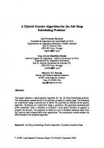
3. GA Representations Cheng, Gen and Tsujimura [7] provide a survey on the different GA representations used for the JSP. They classify them into two categories: direct and indirect. The distinction between direct and indirect representations depends on whether a solution is directly encoded into the genotype or not. Alternatively, in this paper we classify the GA representations for the JSP into two main categories: model-based and algorithm-based. Figure 1 illustrates this classification and lists the available representations in the literature for each category. In model-based representations, the structure of the genotype is based on the definition of the decision variables of a specific JSP mathematical model, and a genotype can be directly interpreted to a feasible or infeasible solution. A special algorithm may be needed to convert infeasible solutions into feasible ones. In model-based representations, optimal solutions are attainable. The existing model-based representations use three types of decision variables: 1) binary decision variables as found in the disjunctive graph model and the ILP model of Manne, 2) processing sequence decision variables as described in the PIAN model, and 3) integer variables representing the operations’ start or completion times. In the binary GA representation, the disjunctive graphbased representation [16] has a large chromosome size and many infeasible solutions are encountered during the GA run, which requires extra computational effort to fix their infeasibilities. This GA representation is excluded from the computational comparison in this paper. In the processing sequence representations, there are three different forms that are based on the processing sequence decision variables as found in the PIAN model. The operation-based (OB) representation [17] uses a single string of genes, where each job is represented by a number of genes equals the number of operations it contains. Based on the order of the operations given in this representation, each operation is assigned the earliest start time permitted by considering the machine availa

1157

bility constraints to generate feasible schedule. In this interpretation mechanism, the technological constraints are easily satisfied. The random keys (RK) representation [18] is very similar to the operation-based one, except that each gene is filled with a randomly generated number between 0 and 1. The random numbers in a given chromosome are sorted out and the resulting order is used to replace these numbers with an integer (the order). Each operation in the studied problem is assigned an integer value so that the resultant string of integers is equivalent to a string of operations. This string is then interpreted into feasible schedule using the same approach as in the operationbased representation with correcting any violation of the technological constraints. The preference list-based (PL) representation, found in [19] and [20], uses a string of operations for each machine instead of a single string for all the operations, which makes it a direct representation of the processing sequence decision variables of the PIAN model. Frequently, violations of the technological constraints are encountered, which requires additional computations to fix it during the interpretation phase. The completion time-based representation [21] uses a string of integer values having a length that equals the total number of operations. The integer value stored in a gene represents the completion time, which equals  si  pi  of its associated operation. This representation requires extra computational effort to fix an expectedly large number of infeasible representations. This representation has been excluded from the computational comparison in this paper. In the algorithm-based representations, the genotype is used to store guiding information to be used by an algorithm to generate feasible schedules, and there is no guarantee for obtaining optimal solutions. In the priority rule-based (PR) representation [22], the chromosome is a string of priority dispatching rules which are applied in sequence to schedule operations within an active schedule generator, namely Giffler and Thompson algorithm [23]. Consequently, the chromosome length equals the total number of operations in a given problem.

GA representations for the JSP

Algorithm-based

Model-based Binary



Disjunctive graph‐based (job  pair relation‐based)  representation [16] 

Processing sequence  Operation‐based (OB) [17] Random keys (RK) [18] Preference list‐based (PL) [19] [20]

Integer Completion time‐based [21]

  

Priority rule‐based (PR) [22] Machine‐based (MB) [22] Job‐based (JB) [23]

Figure 1. Types of GA representations for the JSP. Copyright © 2010 SciRes.

JSEA

1158


In the machine-based (MB) representation [8], the chromosome is a string of machines with a total length equals the number of machines. The sequence of the machines in the chromosome represents the order by which a machine is treated as a bottleneck machine in the shifting bottleneck algorithm [12]. In the job-based (JB) representation [24], the chromosome is a string of jobs with a total length equals the number of jobs. Using the order of the jobs given in the chromosome, a simple algorithm is used to schedule all the operations of the given job in sequence on all the machines at once. To schedule an operation, this algorithm searches for an empty time slot on the assigned machine without violating the technological constraints.

4. Reproduction and Mutation Operators In GA, the reproduction operator can be seen as an approach for conducting neighborhood search; while, mutation operator provides a mechanism to avoid being trapped in a local optima. The design of both operators is crucial for the success of GA. In the literature, the reproduction and mutation operators applied to the JSP are mainly adopted from the literature of applying GA to the traveling salesman problem (TSP). This adoption is motivated by the similarity between the GA representations used for the JSP and the permutation representation used to encode the sequence of visited cities [3]. Among the reproduction operators used in the JSP literature are the partial-mapped crossover (PMX) [25], the order crossover (OX) [26] and the uniform or position-based crossover [27]. For both PMX and OX, there are two versions, one in which there are a single crossover point and another one in which there are two crossover points. The mutation operators used for the JSP implement different mechanisms to exchange the values assigned to randomly selected genes in a given chromosome. Swap mutation, also known as reciprocal exchange mutation, simply exchanges the values assigned to two different randomly selected genes. Inversion mutation, inverts the order of the values assigned to the set of genes located between two randomly selected positions in the chromosome. Insertion or shift mutation selects a gene randomly and sets its value to another randomly selected gene, while the values of the genes between these randomly selected positions are shifted. The displacement mutation is another version of shift mutation in which a substring of genes, instead of a single gene, is moved to a randomly selected new location. Gen and Cheng [3] provide a detailed description of the implementation of the reproduction and mutation operators used in this study.

5. Experimentation, Results and Analysis The previously mentioned GA representations, except the Copyright © 2010 SciRes.

disjunctive graph-based and the completion time-based, are considered in the current computational study. A special computer program prepared in the C++ programming language is used to benchmark the performance of a simple GA implementation with elite preservation strategy. All chromosomes are initialized in a totally random fashion by selecting randomly the values assigned for each gene in the chromosome. In the cases of OB, PL and JB representations, a special attention has been made to avoid operation or job repetitions in the same chromosome. All experiments are conducted with a total number of generations of 300, a fixed population size of 40, a fixed elite size of 5, a fixed mutation probability of 0.1 and reproduction probability of 0.8. For the selection operator, a tournament selector is used. In this selector, two candidate solutions are drawn randomly with a probability proportional to their fitness values, and the one with the highest fitness (lowest makespan) is selected. For each GA representation, the reproduction and mutation operators described in the previous section have been programmed. Since studying the GA performance when different reproduction and mutation operators are used is outside the scope of this paper, we programmed the GA to randomly select an operator from the available list. All reproduction operators have the same probability of being selected, and so the mutation operators. The benchmark problems used in the experimentations are selected 40 standard test problems reported in the literature and made available through the OR-Library in the World Wide Web [28]. All runs are conducted on a personal computer with Intel Pentium Core 2 Duo processor running with a clock speed of 2.67 GHz and RAM of 512 Mega Bytes. For each test problem and GA representation, five GA runs are conducted. The best and average makespan values among the five runs are reported in Table 2. Based on these results, the optimality gap, which is defined as the difference between the best or average makespan value and the lower bound divided by the latter and multiplied by 100, is evaluated for each test problem. Table 3 lists the average among all test problems for both the best and average optimality gaps. From these results, it is clear that the MB representation gives the best quality solutions with a small optimality gap and it is relatively robust with minor variability in the final makespan value among the five runs. This is followed by the PR representation. The OB representation comes in the third place in terms of both the average and best optimality gaps; however its variability in the final makespan value is higher than that of MB and PR representations. The trend of increasing variability is apparent for the remaining GA representations, JB, RK and the worst PL. JSEA


1159

Table 2. Best and average makespan values. GA Representation** Prob.

Size*

No. of Operations

Best known lower bound

OB

RK

PL

Best

Avg.

Best

Avg.

Best

PR

MB

JB

Avg.

Best

Avg.

Best

Avg.

Best

Avg.

abz5

10 x 10

100

1234 (opt.)

1300

1332.2

1327

1373.4

1466

1512

1299

1311.2

1283

1284.8

1425

1443.8

abz6

10 x 10

100

943 (opt.)

1037

1058

1016

1055

1071

1140.2

996

1009.2

967

971.4

1056

1103.8

car1

5 x 11

55

7038 (opt.)

7635

7953.6

7815

8212.8

8675

9306.4

7162

7482.8

7038

7038

7038

7038

car2

4 x 13

52

7166 (opt.)

7638

8014.6

8358

8648.6

8497

9159

7495

7601

7509

7509

7166

7208

car3

5 x 12

60

7312 (opt.)

7973

8156.6

8249

8791.6

9197

10271.6

7543

7794

7543

7543

7312

7346.8

car4

4 x 14

56

8003 (opt.)

8206

8679.4

8894

9258.2

9299

9929.6

8415

8471.2

8423

8423

8003

8003

car5

6 x 10

60

7702 (opt.)

7977

8169.4

8046

8508

9421

9999.6

7840

8018.6

7808

7808

7720

7747.4

car6

9x8

72

8313 (opt.)

8617

9277

9304

9884.4

10530

10999

9083

9257.2

8330

8330

8505

8591.4

car7

7x7

49

6558 (opt.)

6632

6969.2

7084

7430

7526

8305.2

6625

6750.4

6632

6638.6

6590

6600.6

car8

8x8

64

8264 (opt.)

8407

8766.4

9511

9827.2

10022

10635.6

8542

8762

8407

8442.8

8366

8366

la01

5 x 10

50

666 (opt.)

666

688.6

666

682

675

701

671

684.6

666

666

700

720.6

la02

5 x 10

50

655 (opt.)

676

698.8

686

719

715

754

675

692.2

684

684

718

731.2

la03

5 x 10

50

597 (opt.)

631

648

637

655

669

689.6

650

658.4

625

625

645

659.8

la04

5 x 10

50

590 (opt.)

607

629.6

614

623.8

633

695.6

629

667.2

590

590

675

694.4

la05

5 x 10

50

593 (opt.)

593

593

593

593

593

595.6

593

593

593

593

605

622

la06

5 x 15

75

926 (opt.)

926

926

926

934.8

926

931.8

926

937

926

926

941

966.2

la07

5 x 15

75

890 (opt.)

947

963.8

910

945.4

931

971.2

894

930

890

890

903

925.2

la08

5 x 15

75

863 (opt.)

863

881.6

863

886.6

895

922.8

866

877.2

863

863

905

940.4

la09

5 x 15

75

951 (opt.)

951

951

951

955.6

951

966.6

951

958

951

951

1009

1038.6

la10

5 x 15

75

958 (opt.)

958

958

958

958

958

967

958

958.2

958

958

987

1004.8

la11

5 x 20

100

1222 (opt.)

1222

1222

1222

1222

1242

1276.4

1222

1223.8

1222

1222

1264

1271.4

la12

5 x 20

100

1039 (opt.)

1039

1041.4

1039

1051.8

1088

1121.6

1039

1050

1039

1039

1069

1090.8

la13

5 x 20

100

1150 (opt.)

1150

1155.2

1150

1157.8

1189

1201.8

1150

1156.4

1150

1150

1213

1227.6

la14

5 x 20

100

1292 (opt.)

1292

1292

1292

1292

1292

1292

1292

1292

1292

1292

1300

1307.8

la15

5 x 20

100

1207 (opt.)

1274

1294.8

1303

1357.2

1390

1425.4

1274

1304.2

1207

1207

1294

1326.4

la16

10 x 10

100

945 (opt.)

1014

1036.2

1021

1069

1078

1167.4

1003

1034.6

994

996.4

1080

1120.8

la17

10 x 10

100

784 (opt.)

820

865.2

816

861

906

949.2

822

838.4

792

792.4

868

899.2

la18

10 x 10

100

848 (opt.)

933

948

928

961.4

977

1009.6

901

930.8

857

858.2

986

1011.6

la19

10 x 10

100

842 (opt.)

937

965.4

910

946.4

956

1004.4

892

919.2

869

871

980

1014

la20

10 x 10

100

902 (opt.)

989

1018

1035

1047.4

958

1086.2

944

969.4

941

941

980

1055.4

la21

10 x 15

150

1040

1224

1289.6

1230

1286.4

1353

1426.4

1189

1212.2

1105

1120

1285

1310.2

la22

10 x 15

150

927 (opt.)

1078

1135

1074

1160.8

1270

1305.2

1078

1098

963

973.4

1160

1185.8

la23

10 x 15

150

1032 (opt.)

1157

1215.6

1199

1251.6

1332

1348.8

1124

1154

1032

1032

1228

1289.6

la24

10 x 15

150

935 (opt.)

1084

1113.4

1147

1189

1178

1284.8

1059

1094.4

1000

1006

1179

1217.8

la25

10 x 15

150

977 (opt.)

1109

1216.6

1184

1219.2

1270

1357.4

1070

1112.6

1053

1059.4

1174

1213.8

orb1

10 x 10

100

1059 (opt.)

1216

1270.4

1253

1318

1321

1391.4

1106

1152.6

1128

1133.6

1165

1230.2

orb2

10 x 10

100

888 (opt.)

960

1008.4

1001

1030.4

1021

1088.6

939

966

911

911.4

1005

1045.4

orb3

10 x 10

100

1005 (opt.)

1197

1257.2

1200

1244.6

1302

1362.8

1120

1151

1074

1079.2

1176

1186.8

orb4

10 x 10

100

1005 (opt.)

1049

1110.2

1091

1163.4

1158

1252.4

1137

1158.8

1028

1040.6

1202

1234.2

orb5

10 x 10

100

887 (opt.)

1024

1073

1014

1076.8

1120

1178

986

1008.6

911

912.8

980

985.8

* The size of the problem is defined by the number of machines x the number of jobs; ** The acronyms used here for the GA representations are defined earlier in Section 3 and Figure 1, (opt.) means that an optimal solution has been found and the value of the lower bound is the value of the minimum makespan for the given problem.

Copyright © 2010 SciRes.

JSEA



Table 3. Averages of the best and average optimality gaps. Average of Best Optimality Gap %

GA Representation

Average of Avg. Optimality Gap %

OB

6.40

9.90

RK

8.60

12.47

PL

14.79

20.73

PR

5.07

7.35

MB

2.35

2.55

JB

8.95

11.54

50

Average computational time (Seconds)

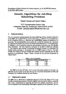
The computational time in seconds is recorded for each run. It is found that the main problem parameter that directly affects the computational time in a given problem is the number of operations. This is mainly attributed to the decoding mechanism of the GA representation used which generally contains a main loop over all the operations of a given problem. This fact is apparent for all representations except MB which is also affected by the number of machines in the decoding algorithm. To illustrate that, all problems that have the same number of operations are sorted out, and the recorded computational time is averaged among those problems. The average computational time is plotted against the number of operations for each GA representation as shown in Figures 2 and 3. The results of OB, RK, PL and JB representations are separated in Figure 2 from those of PR and MB representations for the sake of clarity. It can be concluded from Figures 2 and 3 that the computational time of the GA using OB, RK, PL, JB and PR representations is a polynomial function of the number of operations where this relationship is almost linear for the first four representations as shown in Figure 2. The PR representation employs Giffler and Thompson’s algorithm [23] to interpret the given list of priority rules into an active schedule. This interpretation procedure requires additional computational time in the decoding algorithm, which also depends on the number of operations, resulting in an increasing rate of computational time with the increase of the number of operations. For the MB representation, the computational time is affected by another factor, namely the number of machines, due to the decoding mechanism which employs the shifting bottleneck procedure [12]. This explains the unsteady rate of increase/decrease in the computational time as related only to the number of operations as showin Figure 3. In order to provide a unified measure for comparing the computational time requirements of the GA under the studied six representations, the average computational time in seconds of the five runs divided by the number of operations in a given problem is calculated for all test problems. Then, the average of this measure among all test problems is evaluated for each GA representation, and referred to as the average computational time per operation. This measure is plotted in Figure 4 against the average of the average optimality gap (or simply the average optimality gap) given in Table 3. From Figure 4, it can be concluded that, on average, both RK and PL representations are dominated by the other four representations, and accordingly they may not be considered in the future unless more effective reproduction and mutation operations are devised. MB representation provides the best average optimality gap, while on the other side, job-based (JB) representation is the

45 40 35 30 OB

25 20

RK

15

PL

10

JB

5 0 0

50

100

150

200

No. of operations

Figure 2. Computational time versus number of operations for OB, RK, PL and JB representations. 3000 Average computational time (Seconds)

1160

2500 2000 1500 PR 1000

MB

500 0 0

50

100

150

200

No. of operations

Figure 3. Computational time versus number of operations for PR and MB representations.

Figure 4. Average computational time per operation versus average optimality gap.

JSEA


fastest. The four representations: MB, PR, OB and JB represent the Pareto front from which a software designer may choose.

6. Conclusions In this paper, six different GA representations for the job shop scheduling problem (JSP) are compared. The main two factors that are used in the comparison are the average optimality gap, and the average computational time in seconds divided by the number of operations of a given problem. A set of 40 standard JSP benchmark problems are solved using the GA under the studied six representations, and the averages of both measures are calculated. It is found that the machine-based representation is capable of achieving the lowest optimality gap of 2.55% on average with a small variability among the conducted runs, but with the highest computational time. Both the random keys and preference-list representations are found to be incompetent compared to the other representations.

7. Acknowledgements The author would like to thank an anonymous referee for his/her comments which helped to improve the presentation of the results in this paper.

REFERENCES [1]

J. Holland, “Adaptation in Natural and Artificial Systems,” University of Michigan Press, Ann Arbor, 1975.

[2]

D. E. Goldberg, “Genetic Algorithms in Search, Optimization and Machine Learning,” Addison-Wesley, New York, 1989.

[3]

M. Gen and R. Cheng, “Genetic Algorithms and Engineering Design,” Wiley, New York, 1997.

[4]

M. Pinedo, “Scheduling-Theory, Algorithms, and Analysis,” Prentice-Hall, New Jersey, 2002.

[5]

M. R. Garey, D. S. Johnson and R. Sethi, “The Complexity of Flow Shop and Job-Shop Scheduling,” Mathematics of Operations Research, Vol. 1, No. 2, 1976, pp. 117-129. doi:10.1287/moor.1.2.117

[6]

[7]

[8]

[9]

Y. N. Sotskov and N. V. Shakhlevich, “NP-Hardness of Shop Scheduling Problems with Three Jobs,” Discrete Applied Mathematics, Vol. 59, No. 3, 1995, pp. 237-266. doi:10.1016/0166-218X(93)E0169-Y R. Cheng, M. Gen and Y. Tsujimura, “A Tutorial Survey of Job-Shop Scheduling Problems Using Genetic Algorithms-I. Representation,” Computers and Industrial Engineering, Vol. 30, No. 4, 1996, pp. 983-997. doi:10.1016 /0360-8352(96)00047-2 E. J. Anderson, C. A. Glass and C. N. Potts, “Local Search in Combinatorial Optimization,” Princeton University Press, Princeton, 2003. B. Roy and B. Sussmann, “Les Problemes d’ Ordon-


1161

nancement Avec Constraints Disjonctives,” SEMA, Note D.S., Paris, 1964. [10] T. F. Abdelmaguid, “Permutation-Induced Acyclic Networks for the Job Shop Scheduling Problem,” Applied Mathematical Modeling, Vol. 33, No. 3, 2009, pp. 1560-1572. doi:10.1016/j.apm.2008.02.004 [11] J. Carlier and E. Pinson, “An Algorithm for Solving the Job-Shop Problem,” Management Science, Vol. 35, No. 2, 1989, pp. 164-176. doi:10.1287/mnsc.35.2.164 [12] J. Adams, E. Balas and D. Zawack, “The Shifting Bottleneck Procedure for Job Shop Scheduling,” Management Science, Vol. 34, No. 3, 1988, pp. 391-401. doi:10.128 7/mnsc.34.3.391 [13] H. Bowman, “The Schedule-Sequencing Problem,” Operations Research, Vol. 7, No. 5, 1959, pp. 621-624. doi: 10.1287/opre.7.5.621 [14] H. M. Wagner, “An Integer Linear-Programming Model for Machine Scheduling,” Naval Research Logistics Quarterly, Vol. 6, No. 2, 1959, pp. 131-140. doi:10.1002 /nav.3800060205 [15] A. S. Manne, “On the Job-Shop Scheduling Problem,” Operations Research, Vol. 8, No. 2, 1960, pp. 219-223. doi:10.1287/opre.8.2.219 [16] H. Tamaki and Y. Nishikawa, “A Paralleled Genetic Algorithm Based on a Neighborhood Model and its Application to the Jobshop Scheduling,” Proceedings Of the 2nd International Conference on Parallel Problem Solving from Nature, Amsterdam, 28-30 September 1992, pp. 579-588. [17] M. Gen, Y. Tsujimura and E. Kubota, “Solving Job-Shop Scheduling Problems by Genetic Algorithm,” Proceedings of the IEEE International Conference on Systems, Man and Cybernetics, San Antonio, 2-5 October 1994, pp. 1577-1582. [18] J. Bean, “Genetic Algorithms and Random Keys for Sequencing and Optimization,” ORSA Journal of Computing, Vol. 6, No. 2, 1994, pp. 154-160. [19] L. Davis, “Job Shop Scheduling with Genetic Algorithm,” Proceedings Of the 1st International Conference on Genetic Algorithms, Pittsburgh, 24-26 July 1985, pp. 136-140. [20] F. D. Groce, R. Tadei and G. Volta, “A Genetic Algorithm for the Job Shop Problem,” Computers and Operations Research, Vol. 22, No. 1, 1995, pp. 15-24. doi:10. 1016/0305-0548(93)E0015-L [21] T. Yamada and R. Nakano, “A Genetic Algorithm Applicable to Large-Scale Job-Shop Problems,” Proceedings of the 2nd International Conference on Parallel Problem Solving from Nature, Amsterdam, 28-30 September 1992, pp. 283-292. [22] U. Dorndorf and E. Pesch, “Evolution Based Learning in a Job Shop Scheduling Environment,” Computers and Operations Research, Vol. 22, No. 1, 1995, pp. 25-40. doi:10.1016/0305-0548(93)E0016-M [23] B. Giffler and G. L. Thompson, “Algorithms for Solving Production Scheduling Problems,” Operations Research, Vol. 8, No. 4, 1960, pp. 487-503.

JSEA

1162


[24] C. W. Holsapple, V. S. Jacob, R. Pakath and J. S. Zaveri, “Genetics-Based Hybrid Scheduler for Generating Static Schedules in Flexible Manufacturing Contexts,” IEEE Trans. Systems, Man, and Cybernetics, Vol. 23, No. 4, 1993, pp. 953-971. doi:10.1109/21.247881 [25] D. Goldberg and R. Lingle, “Alleles, Loci and the Traveling Salesman Problem,” Proceedings of the 1st International Conference on Genetic Algorithms and Their Applications, Los Angeles, 1985, pp. 154-159.


[26] L. Davis, “Applying Adaptive Algorithms to Epistatic Domains,” Proceedings of the 9th International Joint Conference on Artificial Intelligence, 1985, pp. 162-164. [27] G. Syswerda, “Uniform Crossover in Genetic Algorithms,” Proceedings of the 3rd International Conference on Genetic Algorithms, San Mateo, 1989, pp. 2-9. [28] J. E. Beasley, “Job Shop Scheduling,” 2008. http://people. brunel. ac.uk/~mastjjb/jeb/orlib/jobshopinfo.html.

JSEA