Department of Computer Science, Meiji University, Kawasaki 214-8571, Japan. Abstract. This paper considers quasi-reduced multi-valued deci- sion diagrams ...
Representations of Logic Functions using QRMDDs Shinobu NAGAYAMA1 , Tsutomu SASAO1;2, Yukihiro IGUCHI3 and Munehiro MATSUURA1 1 Department of Computer Science and Electronics, Kyushu Institute of Technology Iizuka 820-8502, Japan 2 Center of Microelectronics Systems Kyushu Institute of Technology Iizuka 820-8502, Japan 3
Department of Computer Science, Meiji University, Kawasaki 214-8571, Japan
Abstract This paper considers quasi-reduced multi-valued decision diagrams with k bits (QRMDD(k )s) to represent twovalued logic functions. It shows relations between the numbers of nodes in QRMDD(k )s and values of k for benchmark functions; an upper bound on the number of nodes in the QRMDD(k ); difference between the upper bound and the number of nodes in the QRMDD(k )s for random functions; and the amount of total memory, evaluation time, and areatime complexity for QRMDD(k )s. Experimental results using standard benchmark functions show that the area-time complexity takes its minimum when k is between and .
3
6
1. Introduction With the increase of the complexity of digital systems, representations of logic functions that can evaluate functions efficiently and require small amount of memory are becoming important [2]. In this paper, we consider representations of two-valued logic functions using quasi-reduced multi-valued decision diagrams with k bits (QRMDD(k )s). As for methods to represent logic functions by decision diagrams (DDs), binary decision diagrams (BDDs) [1, 7] and multi-valued decision diagrams (MDDs) [3, 10, 12, 14] are known. Especially, MDDs require fewer nodes than corresponding BDDs. Also, the number of memory accesses required in MDDs is smaller than corresponding BDDs [12]. In this paper, we show relations among the amount of memory to represent QRMDD(k ), the number of memory accesses, and values of k. The rest of the paper is organized as follows: In Section 2, we will define MDDs and QRMDDs, and explain benchmark functions and random functions. In Section 3, we obtain an upper bound on the number of nodes in a QRMDD(k ). Also, we show an interesting
property holds for many of benchmark functions. We also show that random functions do not have this property. In Section 4, we introduce the measure called area-time complexity. When we use a QRMDD(k ), the number of memory accesses decreases with k, while the amount of memory to represent it increase with k. We are interested in k that reduces the number of memory accesses without increasing the amount of memory excessively. To obtain such k, we introduce a measure called area-time complexity. By experiments, the measure is the minimum when k is between and .
3
2
6
Definitions
This section defines quasi-reduced multi-valued decision diagrams(QRMDDs), shows a method to represent multiple-output functions, and introduces benchmark functions.
2.1 Representation of Logic Functions
Let f (X ) be a two-valued logic function, where X = (x1; x2; : : : ; xn). Let xi(i = 1; 2; : : :; n) be binary variables, where n = rk. Let X = (X1 ; X2 ; : : : ; Xr ) be a partition of X , where fX g = fX1g [ fX2 g [ : : : [ fXr g and fXi g \ fXj g = �(i 6= j ), and each Xj consists of k binary variables. Then, a two-valued logic function f (X ) can be represented by f (X1 ; X2; : : : ; Xr ): f0; 1; 2; : : :; 2k 1gr ! B , where B = f0; 1g.
2.2 QRMDD
As for the definitions on MDDs, refer [10]. Definition 2.1 The reduced ordered multi-valued decision diagram (RMDD) having non-terminal nodes with k edges is denoted by RMDD(k ). Especially, when k , RMDD( ) is a reduced ordered binary decision diagram (RBDD).
2
1
= 1
Definition 2.2 In a decision diagram (DD), a path from the root node to a terminal node is a path of DD. The number of edges on the path is the length of the path.
Definition 2.3 In a DD, the number of nodes in the DD, denoted by nodes DD , includes terminal nodes.
(
)
( =1 2
f
)
Definition 2.4 When all Xi i ; ; : : :; u appear in this order on an arbitrary path of an MDD(k ), the MDD(k ) is a quasi-reduced multi-valued decision diagram with k bits (QRMDD(k )). The length of an arbitrary path in a QRMDD(k ) is equal to u, the number of input variables. An RMDD has no redundant nodes, while a QRMDD usually has redundant nodes. Therefore, we have the following relation in the number of nodes of an RMDD and its corresponding QRMDD:
(
f
x1 x2
X1
x2 x3
x3
0
=( ( )
)
(
(
( )) =
nodes QRM DD k
() )
u
X
i=1
(
() )
width QRM DD k ; i :
Example 2.1 Consider the function:
= x1x2x3 _ x2x3x4 _ x3x4x1 _ x4x1x2: The RBDD, the RMDD(2), and the QRMDD(2) for f are shown in Fig. 2:1(a), Fig. 2:1(b), and Fig. 2:2, respectively. In Fig. 2:1(a), the solid lines and the broken lines denote 1-edges and 0-edges, respectively. In Fig. 2:1(b), the input variables X = (x1; x2; x3; x4) are partitioned into X = (X1 ; X2), where X1 = (x1; x2) and X2 = (x3 ; x4). We have nodes(RBDD) = 8, nodes(RM DD(2)) = 5, and nodes(QRM DD(2)) = 6. Note that width(QRM DD(2); 2) = 3. (End of Example) f
0,1,2
X2 3
0
1 (a) RBDD
( )) � nodes(QRM DD(k)):
Definition 2.5 Let the input variables be X X1 ; X2 ; : : : ; Xu . Consider a QRMDD for a function f X . The number of non-terminal nodes in the QRMDD with respect to a variable Xi is width of the QRMDD with respect to Xi , and denoted by width QRM DD k ; i . The total number of nodes in the QRMDD(k ) is given by
3 1,2
x4
X2 0
1,2,3
1
2
(b) RMDD( )
Figure 2.1. DDs.
nodes RM DD k
In general, QRMDDs (QRBDDs) require more nodes than corresponding RMDDs (RBDDs). However, QRMDDs (QRBDDs) have the following features: 1. When the RBDDs are too large to be store in the main memory, QRBDDs can be processed much faster than corresponding RBDDs [15]. 2. QRBDDs can be manipulated efficiently by parallel processors [16]. 3. QRBDDs (QRMDDs) are used to design LUT cascades [22]. The most severe limitation of conventional BDDs is their size. When a BDD does not fit in the main memory, the BDD must uses the secondary memory. This will increase the number of page faults, and access to the secondary memory [24]. In such a case, quasi-reduced decision diagrams can be used to reduce the page faults. This approch is useful when the quasi-reduced decision diagram is not so greater than the corresponding reduced decision diagrams.
0
f 0
redundant node
X2
X1
3
1,2
0,1,2
0,1,2,3
0
X2 3
X2 0
1,2,3
1
2
Figure 2.2. QRMDD( ).
2.3 Representations of Multiple-Output Functions Logic networks usually have many outputs. In most cases, independent representation of each output is inefficient. Let the multiple-output functions be F f ; g, and f0 ; f1; : : : ; fm 1 : B n ! B m , where B n and m denote the number of inputs and outputs, respectively. Several methods exist to represent multiple-output functions by using BDDs [13, 18, 19, 20]. In this paper, we use an encoded characteristic function for non-zero output (ECFN) [21] to represent multiple-output functions. In the following, an RBDD means a BDD for an ECFN, and we assume that RMDDs and QRMDDs are generated from these RBDDs.
(
= 10
)
=
2.4 Benchmark Functions
131
In this paper, we use benchmark functions [6, 25] shown in Table 2.1, where n and m denote the number of inputs and outputs, respectively. In this table, the benchmark functions under sequential originally represent sequential circuits. We removed flip-flops(FFs) from sequential circuits to make them combinational. Such functions are renamed by appending ’c’ to the original names. Encodings of BDDs for ECFNs and input variable orderings are obtained in [22]. Details of experimental results are omitted due to the page limitation.
Table 2.1. Benchmark Functions. N ame n m N ame C 432 36 7 f rg1 C 499 41 32 f rg2 C 880 60 26 i1 C 1355 41 32 i2 C 1908 33 25 i3 C 2670 233 140 i4 C 3540 50 22 i5 C 5315 178 123 i6 C 7552 207 108 i7 accpla 50 69 i8 al2 16 47 i9 alcom 15 38 i10 apex1 45 45 ibm apex2 39 3 in1 apex3 54 50 in2 apex5 117 88 in3 apex6 135 99 in4 apex7 49 37 in5 b2 16 17 in6 b3 32 20 in7 b4 33 23 jbp b9 41 21 k2 bc0 26 11 lal bca 26 46 mainpla bcb 26 39 mark1 bcc 26 45 misex2 bcd 26 38 misg c8 28 18 mish cc 21 20 misj chkn 29 7 mlp10 cht 47 36 mux cm150a 21 1 my adder comp 32 3 opa cordic 23 2 pair count 35 16 pcle cps 24 109 pcler8 dalu 75 16 pdc des 256 245 pm1 dk48 15 17 rckl duke2 22 29 rot e64 65 65 sct ex4 128 28 seq example2 85 66 shif t exep 30 63 signet
3
n m N ame n m soar 83 94 spla 16 46 t1 21 23 t2 17 16 table5 17 15 tcon 17 16 term1 34 10 ti 47 72 too large 38 3 ts10 22 16 ttt2 24 21 unreg 36 16 vda 17 39 vg2 25 8 vtx1 27 6 x1 51 35 x3 135 99 x4 94 71 x1dn 27 6 x2dn 82 56 x6dn 39 5 x7dn 66 15 x9dn 27 7 xparc 41 73 sequential s208c 18 9 s298c 17 20 s344c 24 26 s349c 24 26 s382c 24 27 s400c 24 27 s420c 34 17 s444c 24 27 s510c 25 13 s526c 24 27 s641c 54 43 s713c 54 42 s820c 23 24 s832c 23 24 s838c 66 33 s1196c 32 32 s1423c 91 79 s5378c 214 228 s9234c 247 250
28 3 143 139 25 16 201 1 132 6 192 6 133 66 138 67 199 67 133 81 88 63 257 224 48 17 16 17 19 10 35 29 32 20 24 14 33 23 26 10 36 57 45 45 26 19 27 54 20 31 25 18 56 23 94 43 35 14 20 20 21 1 33 17 17 69 173 137 19 9 27 17 16 40 16 13 32 7 135 107 19 15 41 35 19 16 39 8
Number of Nodes in QRMDD(k )
In this part, we first obtain an upper bound on the number of nodes in a QRMDD(k ). Then, we obtain the sizes of QRMDD(k )s for benchmark functions, and show that an interesting property holds for many of them. Finally, we obtain the sizes of QRMDD(k )s for randomly generated logic functions, and show that they can be estimated by the upper bound.
3.1 General Functions
k
1 2 3 4 5 1:00 0:50 0:33 0:25 0:20 0:000 0:014 0:007 0:013 0:009
ave stdv
01
Table 3.2. functions with � � : Name C 499 C 1908 comp i3 in1 mlp10
Circuit error correcting error correcting comparator control control multiplier
Theorem 3.1 An arbitrary n-input logic function can be represented by a QRBDD with at most
1+
r
X
i=0
22
i
N ame my adder pcle tcon vg2 vtx1 x1dn
Circuit adder control control control control control
nodes, where r is the largest integer that satisfies relation
2
r � r:
n
Theorem 3.2 An arbitrary n-input logic function can be represented by a QRMDD(k ) with at most
2sk 1 + t 1 22 2k 1 i=0 X
n
(s+i)k
+2
nodes, where s and t are the smallest integer that satisfy relations n r n s� ; t� s: k k
31
32
The proofs of Theorem : and Theorem : are shown in Appendix.
3.2 Benchmark Functions For each benchmark function in Table 2.1, we counted the number of nodes in QRMDD(k )s for different k. In Table 3.1, ave denotes arithmetic average of the relative sizes, where the number of nodes in QRMDD( ) is set to : , and stdv denotes the standard deviation. We consider the following:
1
�
=1
(
( )) (1))
k � nodes QRM DD k nodes QRM DD
1 00
:
( Since 119 functions out of 131 functions in Table 2.1 satisfy the relation � < 0:1, we have Property 3.1
For arbitrary logic functions, we have the following:
2n r
Table 3.1. Relation of nodes in QRMDD(k ) and k for benchmark functions.
( )) ' k1 nodes(QRM DD(1)) Property 3.1 holds for the 119 functions in Table 2.1. As for remaining 12 functions, � � 0:1 holds. Table 3.2 lists these 12 functions. Note that Table 2.1 does not contain functions (
nodes QRM DD k
having small inputs and outputs.
Table 3.3. The number of nodes in QRMDD(k ) for random functions.
n
10 11 12 13 14 15 16 17 18 19 20
1 249:4 439:1 756:0 1294:8 2318:0 4343:1 8338:5 16167:3 31157:9 58838:4 107222:3
2 103:0 253:2 358:5 598:6 1376:1 1627:0 5348:5 5723:0 19975:9 22107:0 63272:3
k
3 79:0 91:0 298:5 589:2 603:0 843:0 4556:5 4699:0 4939:0 30480:4 37467:0
4 35:0 181:2 274:5 279:0 291:0 531:0 4240:5 4375:0 4387:0 4627:0 45780:3
Table 3.5. Ratio of difference for random functions. n r (%) n r (%) n r (%) 5 1 25:24 12 3 4:81 19 3 10:60 6 2 28:11 13 3 0:48 20 4 18:37 7 2 16:42 14 3 0:30 21 4 4:50 8 2 12:00 15 3 0:68 22 4 0:37 9 2 11:07 16 3 1:54 23 4 0:00 10 2 9:96 17 3 2:96 24 4 0:00 11 3 17:62 18 3 5:71 25 4 0:01
5 35:0 39:0 51:0 286:6 1052:1 1059:0 1063:0 1075:0 1315:0 26852:4 33827:0
4
When we use QRMDD(k ), the amount of memory access decreases with k, while the total amount of memory increases with k. Thus, we are interested in finding k that reduces the number of memory access without increasing the total amount of memory excessively. To obtain such k, we introduce a measure called area-time complexity.
Table 3.4. Upper bound on the number of nodes in QRMDD(k )s.
n
10 11 12 13 14 15 16 17 18 19 20
1 277 533 789 1301 2325 4373 8469 16661 33045 65813 131349
2 103 347 359 603 1383 1627 5479 5723 21863 22107 87399
3.3 Random Functions
k
3 79 91 331 591 603 843 4687 4699 4939 37455 37467
4 35 275 275 279 291 531 4371 4375 4387 4627 69907
31
4.1 Model of Computation
5 35 39 51 291 1060 1059 1063 1075 1315 33828 33827
We assume the followings: 1. MDDs are implemented directly, not simulated by using BDD packages [10]. 2. Encoded input values are available as inputs, and their access time is negligible. For example, when X1 x1; x2; x3; x4 ; ; ; , X1 is available as an input. 3. Access to the MDD nodes is time-consuming.
(
2
10
1
) = (1 0 0 1)
=9
=
In this case, the computation time is proportional to the number of access to the MDD nodes.
We examined whether Property : holds for random functions. For each n, we randomly generated n 1 minterms. Table 3.3 shows average numbers of nodes in QRMDD(k )s for n-input random functions. For each n, we generated samples. The deviation of each data is within � of the averages. Table 3.4 shows upper bounds on the numbers of nodes in QRMDD(k )s derived from Theorem 3.2. The ratio of difference between upper bounds and experimental results on the number of nodes in QRMDD( ) for n-input random functions is computed as follows:
2%
Area-Time Complexity of QRMDD(k )
experimental result = upper boundupper � 100 bound
Table 3.5 shows that is large after r changes, and is small in other cases. This means that the size of QRMDD(k ) for randomly generated functions can be estimated by Theorem 3.2. Table 3.3 also shows that Property 3.1 doesn’t hold for random functions. This fact shows that benchmark functions have quite different property from random functions.
4.2 Amount of Memory to Represent QRMDD(k) Because QRMDD(k ) evaluates variables X1 ; X2; : : : ; Xu in this order, we can use a counter to obtain the next variable to evaluate. Therefore, when a QRMDD(k ) is stored in a memory, we need not store an index in a node, but have only to store the next addresses. On the other hand, in an RMDD(k ), we have to store an index and the next addresses because the next variable to evaluate may be different in different paths.
41
42
Example 4.1 Fig. : and Fig. : illustrate data structures of a node in a QRMDD( ) and an RMDD( ), respectively. (End of Example)
2
2
Because each node in a QRMDD(k ) has need k nodes QRM DD k
2
(
2k edges, we
( ))
words to represent all nodes in a QRMDD(k ). When a DD is stored in a memory, each node requires a unique address. The number of bits necessary to specify the address of a node is dlog2 nodes DD e:
(
)
Xi 0
1
2
3
Table 4.2. Relation of k and AT for QRMDD(k ) for benchmark functions.
Memory - edge address - edge address - edge address - edge address
0 1 2 3
(a)
k
ave stdv
(b)
Figure 4.1. Data structure of a node in QRMDD( ).
2
Xi 0
1
2
3
Memory index - edge address - edge address - edge address - edge address
0 1 2 3
(a)
(b)
Figure 4.2. Data structure of a node in RMDD( ).
2
Therefore, the total amount of memory to represent a QRMDD(k ) is
2knodes(QRM DD(k))dlog2 nodes(QRM DD(k))e:
1 2 3 4 5 1:00 0:46 0:39 0:43 0:53 0:000 0:019 0:027 0:032 0:047
Table 4.3. Relation of k and AT 2 for QRMDD(k ) for benchmark functions. k
ave stdv
1 2 3 4 5 6 7 1:000 0:233 0:133 0:112 0:113 0:131 0:166 0:000 0:011 0:011 0:011 0:014 0:023 0:029
In this paper, the area corresponds to the necessary amount of memory to represent a QRMDD(k ), and the time corresponds to the number of memory accesses to evaluate it. The measure AT is used when both the amount of memory and the number of memory accesses are equally important. On the other hand, the measure AT 2 is used when the number of memory accesses is more important than the amount of memory. For example, AT can be used for embedded systems [2], while AT 2 can be used for logic simulators [8, 9].
4.4 Experimental Results 4.3 Area-Time Complexity of QRMDD(k)s
Because a QRMDD(k ) evaluates k variables at a time, the number of memory accesses of a QRMDD(k ) is k1 of the corresponding QRMDD( ). On the other hand, the amount of memory necessary to store a QRMDD(k ) node increases with k . In this section, we consider the area-time complexity [5, 23] for QRMDD(k ) and obtain the k that minimizes the area-time complexity.
1
2
Definition 4.1 The area-time complexity is the measure of computational cost considering both area and time. It is defined by AT area � time ;
=(
or
AT 2
) (
)
= (area) � (time)2 :
Table 4.1. Relation of k and A for QRMDD(k ) for benchmark functions. k
ave stdv
1 2 3 4 5 1:00 0:91 1:14 1:65 2:54 0:000 0:036 0:070 0:114 0:190
For each benchmark function in Table 2.1, we obtained three measures A, AT , and AT 2 . Table 4.1, Table 4.2, and Table 4.3 show the relation of k and A, AT , and AT 2 , respectively. In these tables, ave denotes the arithmetic average, and stdv denotes the standard deviation for benchmark functions. For each benchmark function in Table 2.1, A takes its minimum when k ; AT takes its minimum when k or k ; and AT 2 takes its minimum when k � .
=2
=4
=3
=4 6
4.5 Analysis for the Functions that Satisfy Property 3.1
44
In Section : , for QRMDD(k )s, we found values of k that make A, AT and AT 2 minimum, experimentally. In this section, we assume that Property 3.1 holds, and will find the values k that make A, AT and AT 2 minimum, analytically. Let A and T be the necessary amount of memory to represent a QRMDD(k ), and the number of memory accesses necessary to evaluate a QRMDD(k ), respectively. Then, we have the following:
A
= 2k nodes(QRM DD(k))dlog2 nodes(QRM DD(k))e; T
= d nk e:
(
Let assume that Property 3.1 holds and nodes QRM DD
(1)) = N . Then we have: N 2k A ' N dlog2 e; k
AT and
AT 2
'
k
2kn N dlog2 N e; k2 k
' 2kn3 N dlog2 Nk e: k 2
Note that N is usually greater than a few hundreds, while k is usually at most . Thus, we can use the following approximation:
7
dlog2 N
log2 ke ' dlog2 N e:
Therefore, A, AT and AT 2 can be simplified to
A'
2k C0; k
AT
' 2k2 C1; k
and AT 2
' k2 3 C2 ; k
respectively, where the constants C0 , C1 and C2 are independent of k. From the above formulas, we can see that A, AT and AT 2 take their minimum when k ,k and k , respectively.
=4
5
=2 =3
Conclusion and Comments
In this paper, we considered a method to represent logic functions by using QRMDD(k )s. Especially, 1) We derived an upper bound on the number of nodes in a QRMDD(k ), and showed that the numbers of nodes in QRMDD(k )s for random functions can be estimated by the bound, 2) We showed that Property 3.1 holds for many benchmark functions, and 3) We showed that the area-time complexity for QRMDD(k ) takes its minimum when k � , and 4) We showed that benchmark functions have quite different property from randomly generated functions.
=3 6
Acknowledgments This research is partly supported by the Grant in Aid for Scientific Research of The Japan Society for the Promotion of Science (JSPS), and the Takeda Foundation.
References [1] P. Ashar and S. Malik, “Fast functional simulation using branching programs,” ICCAD’95, pp. 408–412, Nov. 1995. [2] F. Balarin, M. Chiodo, P. Giusto, H. Hsieh, A. Jurecska, L. Lavagno, A. Sangiovanni-Vincentelli, E. M. Sentovich, and K. Suzuki, “Synthesis of software programs for embedded control applications,” IEEE Trans. CAD, Vol. 18, No. 6, pp.834-849, June 1999. [3] B. Becker and R. Drechsler, “Efficient graph based representation of multi-valued functions with an application to genetic algorithms,” Proc. of International Symposium on Multiple Valued Logic, pp. 40-45, May 1994. [4] R. K. Brayton, “The future of logic synthesis and verification,” in S. Hassoun and T. Sasao (eds.) Logic Synthesis and Verification, Kluwer Academic Publisher, 2001 pp. 408-434.
[5] R. P. Brent and H. T. Kung, “The area-time complexity of binary multiplication,” Journal of the ACM, Vol. 28, No. 3, pp. 521-534, July 1981. [6] F. Brglez and H. Fujiwara, “Neutral netlist of ten combinational benchmark circuits and a target translator in FORTRAN,” Special session on ATPG and fault simulation, Proc. IEEE Int. Symp. Circuits and Systems, June 1985, pp. 663-698. [7] R. E. Bryant, “Graph-based algorithms for boolean function manipulation,” IEEE Trans. Comput., Vol. C-35, No. 8, pp. 677–691, Aug. 1986. [8] Y. Iguchi, T. Sasao, M. Matsuura, and A. Iseno “A hardware simulation engine based on decision diagrams,” Asia and South Pacific Design Automation Conference (ASPDAC’2000), Yokohama, Japan, Jan. 26-28, 2000, pp. 73-76. [9] Y. Iguchi, T. Sasao, M. Matsuura, “Implementation of multiple-output functions using PQMDDs,” Proc. of International Symposium on Multiple-Valued Logic, pp. 199-205, May 2000. [10] T. Kam, T. Villa, R. K. Brayton, and A. L. SangiovanniVincentelli, “Multi-valued decision diagrams: Theory and Applications,” Multiple-Valued Logic, 1988, Vol. 4, No. 1-2, pp. 9–62, 1998. [11] H.-T. Liaw, and C.-S. Lin. “On the OBDD-representation of general Boolean function,” IEEE Transactions on Computers, Vol. 4, No. 6, pp. 661–664, June 1992. [12] P. C.McGeer, K. L. McMillan, A. Saldanha, A. L. Sangiovanni-Vincentelli, and P. Scaglia, “Fast discrete function evaluation using decision diagrams,” ICCAD’95, pp. 402–407, Nov. 1995. [13] S. Minato, N. Ishiura, and S. Yajima, “Shared binary decision diagram with attributed edges for efficient Boolean function manipulation,” Proc. 27th ACM/IEEE Design Automation Conf., pp. 52–57, June 1990. [14] D. M Miller, “Multiple-valued logic design tools,” Proc. of International Symposium on Multiple Valued Logic, pp. 2– 11, May 1993. [15] H. Ochi, K. Yasuoka and S. Yajima, “Breadth-first manipulation of very large binary-decision diagrams,” 1993 IEEE/ACM International Conference on Computer-Aided Design, pp. 48-55, Nov. 1993. [16] H. Ochi, N. Ishiura and S. Yajima, “Breadth-first manipulation of SBDD of Boolean function for vector processing,” 28th ACM/IEEE Design Automation Conference, pp. 413416, 1991. [17] T. Sasao, “FPGA design by generalized functional decomposition,” (Sasao ed.) Logic Synthesis and Optimization, Kluwer Academic Publishers, 1993, pp. 233-258. [18] T. Sasao and M. Fujita (eds.), Representations of Discrete Functions, Kluwer Academic Publishers 1996. [19] T. Sasao and J. T. Butler, “A method to represent multipleoutput switching functions by using multi-valued decision diagrams,” Proc. of International Symposium on MultipleValued Logic, pp. 248-254, Santiago de Compostela, Spain, May 29-31, 1996. [20] T. Sasao, Switching Theory for Logic Synthesis, Kluwer Academic Publishers, 1999.
where
X1
(
2
2
r 0
1
)
[21] T. Sasao, “Compact SOP representations for multiple-output functions: An encoding method using multiple-valued logic,” Proc. of International Symposium on MultipleValued Logic, Warsaw, Poland, May 22 - 24, 2001, pp. 207211. [22] T. Sasao, M. Matsuura, and Y. Iguchi, “Cascade realization of multiple-output function and its application to reconfigurable hardware,” International Workshop on Logic and Synthesis, Lake Tahoe, June 2001, pp. 225-230. [23] C. D. Thompson, “Area-Time Complexity for VLSI,” Ann. Symp. on Theory of Computing, May 1979 pp. 81-89. [24] I. Wegener, Branching Programs and Binary Decision Diagrams: Theory and Applications, SIAM 200.
A.1 Proof of Theorem 3.1 Definition A.1 Suppose that a quasi-reduced ordered binary decision diagram (QRBDD) for an n-input logic function is partitioned into two parts as shown in Fig A: . It is partitioned into the upper part and the lower part. The upper part has the variables X1 = x1; x2; : : : ; xn r , while the lower part has the variables X2 = xn r+1 ; : : : ; xn .
(
1 )
(
)
Proof of Theorem 3.1 The number of non-terminal nodes . This in the complete binary tree for n variables is n gives the number of nodes in the upper part. As for the lower part, the width of QRBDD becomes narrow because the nodes representing the same functions are deleted. The upper bound on the number of nodes in a BDD becomes minimum when r is the maximum integer satisfying n r � r [11]. As for the lower part, at most 2r r-input logic functions are represented. When all of these functions are represented, the number of nodes in the lower part becomes maximum. In this case, the BDD represents the logic function as follows:
2
2
2
)=
_
~ai 2Bn
) )
r
( =0
1+
r
X
i=0
)
22 : i
(Q.E.D) First, we will consider Lemma A.1 to prove Theorem 3.2.
( )
Lemma A.1 Let an n-input logic function be f X , where X x1; x2; : : : ; xn . Let f X be decomposed as
=(
)
( )
( ) = gi(h(X1; X2; : : :; Xi); Xi+1; : : : ; Xu); where u = d nk e, and let �i be the column multiplicity of the decomposition for i = 1; 2; : : :; u. Then, the number of f X
nodes in the QRMDD(k ) for f is given by
(
( )) =
nodes QRM DD k
u
X
i=1
�i :
Proof Since the width of the QRMDD(k ) with respect to a variable Xi is equal to the column multiplicity �i [17, 18], we have the lemma. (Q.E.D)
Appendix
(
( (
A.2 Proof of Theorem 3.2
[25] S. Yang, Logic synthesis and optimization benchmark user guide version 3.0, MCNC, Jan. 1991.
f X1 ; X2
�
2n
Figure A.1. Partition of BDD.
A
(X1 = ~ai) = 10 (otherwise ):
The upper part realizes X1~ai , and the lower part realizes f ~ai ; X2 .r Because f ~ai ; X2 is an r-input logic function, at most 2 different f ~ai ; X2 exist in the lower part. When 2i functions are realized for each i i ; : : :; r from the terminal node to the r, the QRBDD has the maximum number of nodes. Therefore, the number of nodes in a QRBDD is at most
n-r
X2
X1~ai
r
X1~ai f ~ai ; X2 ;
(
)
1
Proof of Theorem 3.2 By Lemma A.1, the number of nodes in a QRMDD(k ) for an n-input logic function is equal to the sum of the column multiplicities that are obtained by iterative functional decompositions. The upper part of the QRBDD is decomposed into s parts. In this case, �1; �2 ; : : :; �s are ; k; 2k; : : : ; sk. It is a geometric progression with the initial term and the common ratio k . The lower part of the QRBDD is decomposed into t parts. Also in the lower part, the number of nodes is equal to the sum of the column multiplicities. In other words, it is equal to the sum of the widths of a QRBDD with respect to corresponding variables. When n 6 s t k, the number of variables in Xu is not a multiple of k. So, the column multiplicity for this part is computed separately. Note that �u , since f is a two-valued logic function. Thus, the number of nodes in QRMDD(k) is at most
12 2
1
2
2
=( + )
=2
2sk 1 + t 1 22 2k 1 i=0 X
n
(s+i)k
+ 2: (Q.E.D)