EVMDDs can produce fast and compact elementary func- tion generators. 1. ..... put variable (x1 x0 y1)2 = (101)2 and the initial mask data. (111)2 is computed to ...
Representations of Two-Variable Elementary Functions Using EVMDDs and Their Applications to Function Generators Shinobu Nagayama
Tsutomu Sasao
Department of Computer Engineering, Hiroshima City University Hiroshima 731-3194, Japan
Department of Computer Science and Electronics, Kyushu Institute of Technology Iizuka 820-8502, Japan
Abstract This paper proposes a method to represent two-variable elementary functions using edge-valued multi-valued decision diagrams (EVMDDs), and presents a design method and an architecture for function generators using EVMDDs. To show the compactness of EVMDDs, this paper introduces a new class of integer-valued functions, l-restricted Mp-monotone increasing functions, and derives an upper bound on the number of nodes in an edge-valued binary decision diagram (EVBDD) for the l-restricted Mp-monotone increasing function. EVBDDs represent l-restricted Mpmonotone increasing functions more compactly than MTBDDs and BMDs when p is small. Experimental results show that all the two-variable elementary functions considered in this paper can be converted into l-restricted Mpmonotone increasing functions with p 1 or p 3, and can be compactly represented by EVBDDs. Since EVMDDs have shorter paths and smaller memory size than EVBDDs, EVMDDs can produce fast and compact elementary function generators.
1. Introduction Elementary functions have wide applications including computer graphics and digital signal processing, and various circuits (function generators) for them have been developed [16]. However, most existing methods are intended for one-variable elementary functions [5, 14, 19, 20, 24–26], and only a few methods exist for multi-variable elementary functions [7, 8, 29]. As far as we know, no study on graph-based representations for multi-variable elementary functions has been presented. This paper proposes a method to represent two-variable elementary functions using EVMDDs, and presents an architecture and a design method for function generators. To analyze complexities for two-variable elementary functions, this paper introduces a new class of integer-valued functions, l-restricted Mp-monotone increasing functions, and
derives an upper bound on the number of nodes in an edgevalued binary decision diagram (EVBDD) for the function. Theoretical analysis and experimental results show that EVMDDs can compactly represent both one- and twovariable elementary functions, and our function generators using EVMDDs can compactly realize such functions with the same architecture. This paper is organized as follows: Section 2 introduces a fixed-point representation to convert a real-valued elementary function into an integer-valued function, and decision diagrams used in this paper. Section 3 considers representations of two-variable elementary functions using decision diagrams. It introduces an l-restricted Mp-monotone increasing function, and derives an upper bound on the number of nodes in an EVBDD for the function. Section 4 presents an architecture and a design method for function generators based on EVMDDs. And, Section 5 concludes the paper. Proofs of theorems are omitted because of the page limitation.
2. Preliminaries
��� ������ � ���� � �� � � �������� Definition 1 Let B 0 1�, Z be the set of the integers, and R be the set of the real numbers. An n-input m-output logic function is a mapping: Bn � Bm , an integer-valued function is Bn � Z, and a two-variable real function is R � R � R. Definition 2 The binary fixed-point representation of a number is denoted by X �xn int 1 xn int 2 � � � x1 x0 � x 1 x 2 � � � x n f rac �2 , where xi � 0 1�, n int is the number of bits for the integer part, and n f rac is the number of bits for the fractional part of X. This is the two’s complement representation. In this paper, X � denotes the set of binary variables in X. Definition 3 Precision is the total number of bits for a binary fixed-point representation. Specially, n-bit precision
(a) Table for 2-D norm.
X 0.00 0.00 0.00 0.00 0.25 0.25 0.25 0.25 0.50 0.50 0.50 0.50 0.75 0.75 0.75 0.75
Y 0.00 0.25 0.50 0.75 0.00 0.25 0.50 0.75 0.00 0.25 0.50 0.75 0.00 0.25 0.50 0.75
Norm 0.00 0.25 0.50 0.75 0.25 0.35 0.56 0.79 0.50 0.56 0.71 0.90 0.75 0.79 0.90 1.06
Y 0.00 0.01 0.10 0.11 0.00 0.01 0.10 0.11 0.00 0.01 0.10 0.11 0.00 0.01 0.10 0.11
fb 0.00 0.01 0.10 0.11 0.01 0.01 0.10 0.11 0.10 0.10 0.11 1.00 0.11 0.11 1.00 1.00
X 00 00 00 00 01 01 01 01 10 10 10 10 11 11 11 11
Y 00 01 10 11 00 01 10 11 00 01 10 11 00 01 10 11
f 0 1 2 3 1 1 2 3 2 2 3 4 3 3 4 4
specifies that n bits are used to represent the number; that is, n n int � n f rac. In this paper, an n-bit precision function f �X Y � means that both of the input variables X and Y have n-bit precisions1 . By fixed-point representation, we can convert an nbit precision two-variable real function into a 2n-input moutput logic function. The logic function can be converted into an integer-valued function by considering binary vectors as integers. That is, we can convert an n-bit precision two-variable real function into an integer-valued function: B2n � Pm , where Pm 0 1 � � � 2m � 1�. In this paper, twovariable elementary functions are converted into integervalued functions by using fixed-point representation, unless stated otherwise. And, for simplicity, x0 and y0 denote the least significant bits in the fixed-point representations of X and Y , respectively. Example 1 Table 1 (a) is the function table for the Euclidean norm function for a two-dimensional vector: � X 2 � Y 2 . The 2-bit precision fixed-point representation of this function is the logic function fb �X Y � in Table 1 (b). By converting output vectors into integers, we have the integer-valued function f �X Y � of fb �X Y � in Table 1 (c). In this paper, the 2-bit precision 2-D norm function denotes the integer-valued function f �X Y � in Table 1 (c). (End of Example)
� � ������� �������� This subsection defines decision diagrams used in this paper. For more detail on definition and reduction rules of each decision diagram, see [6, 22, 31, 32]. 1 Although
xi
the precision for function values can be different from the precision of the inputs, in this paper, we assume that the number of fractional bits for function values is n. Thus, function values have (n int � n)bit precision, where n int is the number of integer bits for function values.
xi
xi α 1− α 0
(b) Table for fb �X Y �. (c) Table for f �X Y �.
X 0.00 0.00 0.00 0.00 0.01 0.01 0.01 0.01 0.10 0.10 0.10 0.10 0.11 0.11 0.11 0.11
α0
α0
Table 1. Tables for 2-bit precision 2-D norm function. α0
α1
0
(a) Terminal case.
0
α0
xj
xi α1
α 1− α 0
xj
xj
xj
(b) Non-terminal case.
Figure 1. Conversion of an MTBDD node into an EVBDD node. Definition 4 A binary decision diagram (BDD) [2, 15] is a rooted directed acyclic graph (DAG) representing a logic function. The BDD is obtained by repeatedly applying the Shannon expansion f xi f0 � xi f1 to the logic function. It consists of two terminal nodes representing function values 0 and 1 respectively, and non-terminal nodes representing input variables. Each non-terminal node has two unweighted outgoing edges, 0-edge and 1-edge, that correspond to the values of the input variables. Both terminal nodes have no outgoing edges. Definition 5 A multi-terminal BDD (MTBDD) [4] is an extension of a BDD, and represents an integer-valued function. In the MTBDD, the terminal nodes are labeled by integers. Definition 6 A binary moment diagram (BMD) [3] is a rooted DAG representing an integer-valued function. The BMD is obtained by repeatedly applying the arithmetic transform expansion f f0 � xi � f1 � f0 � to the integervalued function. The BMD consists of terminal nodes representing the arithmetic coefficients, and non-terminal nodes representing the arithmetic transform expansions. Each non-terminal node has two edges corresponding to two terms: f0 and xi � f1 � f0 � in the arithmetic transform expansion. Definition 7 An edge-valued BDD (EVBDD) [12, 13] is a variant of a BDD, and represents an integer-valued function. The EVBDD is obtained by repeatedly applying the expansion f xi f0 � xi � f1� � α� to the integer-valued function, where f1 f1� � α, and α is the constant term of f1 . The EVBDD consists of only one terminal node representing 0 and non-terminal nodes with 1-edges having integer weights α. In the EVBDD, 0-edges always have zero weights, and the incoming edge into the root node can have a non-zero weight. In a reduced EVBDD, each node represents a distinct sub-function. An EVBDD is obtained from an MTBDD by recursively applying the conversion shown in Fig. 1 to each non-terminal node in an MTBDD, where in Fig. 1, dashed lines and solid lines denote 0-edges and 1-edges, respectively. Definition 8 For an n-bit precision number X, if X � Xu � � Xu 1 � � � � � � X1 �, Xi � � φ, and Xi � X j �
x1
xi
Xi
α2
xj
0
x0
α1
α3
α2
f1
f2
f3
f0
f1
f2
y1
x1
y1
1
A
y1
1 A x0
A
1
y1 y1
A
A
1
1
α 2+ α 3
y0 f0
y1
A
1 A x0
x0
3
2
y1
xj α1
1
1
y0
y0
f3 0 1
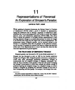
Figure 2. Conversion of EVBDD nodes into an EVMDD node. φ �i � j�, then �Xu Xu 1 � � � X1 � is a partition of X. Each Xi forms a super variable. Let Xi ki and ku � ku 1 � � � � � k1 n. Then, by considering each super variable as a multivalued variable, an integer-valued function f �X � : Bn � Z can be converted into a multi-valued input integer function f �Xu Xu 1 � � � X1 � : Pu � Pu 1 � � � � � P1 � Z, where 0 1 2 � � � 2ki � 1�. Pi Definition 9 A multi-valued decision diagram (MDD) is a rooted DAG representing a multi-valued input integer function. The MDD is obtained by repeatedly applying the Shannon expansion to the multi-valued input integer function [11]. It consists of terminal nodes representing function values and non-terminal nodes representing multivalued variables. Each non-terminal node has multiple unweighted outgoing edges that correspond to the values of multi-valued variable. When an MDD represents a function for which multi-valued variables have different domains, it is a heterogeneous MDD [17, 18]. In the following, the heterogeneous MDD is simply denoted by the MDD. Definition 10 An edge-valued MDD (EVMDD) is an extension of an MDD, and represents a multi-valued input integer function. It consists of one terminal node representing 0 and non-terminal nodes with edges having integer weights, and 0-edges always have zero weights. As shown in Fig. 2, an EVMDD is obtained by merging non-terminal nodes in an EVBDD according to the partition of X. Example 2 Fig. 3 (a), (b), (c), and (d) show the MTBDD, the BMD, the EVBDD, and the EVMDD for the 2-bit precision 2-D norm function in Table 1 (c), respectively. Note that for readability of the figures, several terminal nodes are not shared. In Fig. 3 (a) and (c), dashed lines and solid lines denote 0-edges and 1-edges, respectively. Note that the EVBDD has weighted 1-edges. In Fig. 3 (b), ‘A’ in a circle denotes the arithmetic transform expansion. And, in Fig. 3 (d), the set of binary variables X � � Y � is partix1 x0 y1 � and X1 � y0 �. To obtioned into X2 � tain the function value 3 for X �10�2 and Y �10�2 , in the MTBDD, we traverse the MTBDD from the root node to a terminal node according to the input values, and obtain the function value from the terminal node. In the BMD,
2 3
1
1
4
3
0
A
y0 1
1 2
A
1
y0 1
-1 -1
(a) MTBDD
A
y0 1
A
1 2
y0 1
-1
y1 A
1
y0
-2
(b) BMD
x1 2
x0 y1
X2 0 7 1 3 5 2 4 6 2 2 3
x0 1
y1
1
y1
2 1
1
y0
0
1
0
(c) EVBDD
X1
1
2 2
4
1 1
0 (d) EVMDD
Figure 3. Four types of decision diagrams for the 2-bit precision 2-D norm function. we obtain the function value by computing the arithmetic transform expansion f f0 � xi � f1 � f0 � recursively at each non-terminal node. And, in the EVBDD and the EVMDD, we obtain the function value as the sum of the weights for the edges traversed from the root node to the terminal node. Note that we traverse the EVMDD using X2 5 and X1 0. (End of Example)
3. Graph-Based Representations of TwoVariable Elementary Functions This section introduces an l-restricted Mp-monotone increasing function, and derives an upper bound on the number of nodes in an EVBDD for the l-restricted Mpmonotone increasing function. Experimental results in this section show that EVBDDs for two-variable elementary functions are more compact than MTBDDs and BMDs for them.
���� l ���� ��� �� � p��� � � � � ������ � �� � �� � Definition 11 An n-bit precision integer-valued function f �X � such that 0 � f �X � 1� � f �X � � p and f �0� 0 is a totally Mp-monotone increasing function (or simply, Mp-monotone increasing function). That is, for an Mpmonotone increasing function f �X �, f �0� 0, and the increment of X by one increases the value of f �X � by at most p.
Definition 12 An n-bit precision integer-valued function f �X � is an l-restricted Mp-monotone increasing function when for 1 � l � n, all the l-bit precision subfunctions g�Xl � of f are Mp-monotone increasing functions, where g�Xl � f ��a Xl �, X � xn 1 xn 2 � � � x0 �, Xl � xl 1 xl 2 � � � x0 �, and �a is an assignment to �xn 1 xn 2 � � � xl �2 . Theorem 1 For an n-bit precision l-restricted Mpmonotone increasing function f �X �, the number of nodes in the EVBDD is at most 2n
l
l
� ∑ � p � 1�2
i
1
�l
(1)
i 1
where l is the largest integer satisfying 2n l � p � 1�2 1 , and the variable order of the EVBDD is xn 1 xn 2 � � � x0 (from the root node to the terminal node). l
Note that the upper bound for l-restricted Mp-monotone increasing functions shown in Theorem 1 is equal to the upper bound for totally Mp-monotone increasing functions shown in [19]. Example 3 Consider a 16-bit precision l-restricted Mpmonotone increasing function. When p 1, l 3, and the upper bound given by (1) is 8 327. When p 3, l 2, and (End of Example) the upper bound is 16 450. Definition 13 An n-bit precision integer-valued function f �X � is an extended l-restricted Mp-monotone increasing function when for 1 � l � n, all the l-bit precision sub-functions of f are Mp-monotone increasing functions g�Xl � or represented by g�Xl � � b, where a sub-function xn 1 xn 2 � � � x0 �, is f ��a Xl �, b is an integer, X � Xl � xl 1 xl 2 � � � x0 �, and �a is an assignment to �xn 1 xn 2 � � � xl �2 . Lemma 1 Let f �X � be an extended l-restricted Mpmonotone increasing function. For any integer l � satisfying 1 � l � � l, f �X � is an extended l � -restricted Mp-monotone increasing function. Lemma 2 Let f �X � be an l-restricted Mp-monotone increasing function, and let g�X � be an extended l-restricted Mp-monotone increasing function which is obtained by adding constant values to l-bit precision sub-functions of f . Then, the EVBDDs for f �X � and g�X � have the same number of nodes. Corollary 1 Let f �X � be an extended l-restricted Mpmonotone increasing function, and let g�X � be a linear transformation of f : g�X � a f �X �� b, where a and b are integers. Then, the EVBDDs for f �X � and g�X � have the same number of nodes.
Table 2. Function tables for 2-bit precision two-variable functions. X (a) Table for 2-D norm. (b) Table for Y �1 . X X Y 0 1 2 3 Y 0 1 2 3 0 0 1 2 3 0 0 1 2 3 1 1 1 2 3 1 0 1 2 2 2 2 2 3 4 2 0 1 1 2 3 3 3 4 4 3 0 1 1 2
(c) Table for g�Z �. x1 x0 y1 y0 00 01 10 11 00 0 -1 -2 -3 01 0 -1 -2 -2 10 0 -1 -1 -2 11 0 -1 -1 -2
�� � ������������ ����� �� �� � �� � As shown in Section 2, n-bit precision two-variable elementary functions can be converted into 2n-bit precision integer-valued functions. That is, n-bit precision twovariable functions f �X Y � can be converted into 2n-bit precision one-variable functions f �Z �, where Z
2n X � Y
�xn
1 xn 2
���
x0 yn
1 yn 2
���
y0 �2 �
When f �Z � is an l-restricted Mp-monotone increasing funcl tion for the largest integer l satisfying 22n l � p � 1�2 1 , Theorem 1 gives the upper bound on the number of nodes in an EVBDD for f �X Y �. Example 4 As�shown in Table 2 (a), the 2-bit precision 2-D norm function X 2 � Y 2 can be converted into the extended 2-restricted M1-monotone increasing function f �Z �. Note that in the table, values increase by at most one for each column. Similarly, the 2-bit precision two-variable function X Y �1 shown in Table 2 (b) can be converted into a linear transformation of the extended 2-restricted M1-monotone increasing function g�Z � shown in Table 2 (c): �1 � g�Z �. (End of Example) From here, we are going to show some classes of twovariable elementary functions whose EVBDDs are small. Lemma 3 Let h�Y � be an n-bit precision Mp-monotone increasing function. Then, for arbitrary one-variable function g�X �, two-variable functions f �X Y � g�X �� h�Y � are the extended n-restricted Mp-monotone increasing functions. Lemma 4 Let h�Y � be an n-bit precision Mp-monotone increasing function. Then, for arbitrary one-variable function g�X �, two-variable functions f �X Y � g�X � � h�Y � can be converted into a linear transformation of the extended nrestricted Mp-monotone increasing functions. Lemma 5 Let h�Y � be an n-bit precision Mp-monotone increasing function, and let g�X � be a real function satisfying 0 � g�X � � 1. Then, an n-bit precision two-variable function f �X Y � g�X � h�Y � is an n-restricted Mp-monotone increasing function. In Lemma 5, if the dynamic range of g�X � is large, then the EVBDD can be large. For example, the n-bit multiplier requires O(2n) nodes [31].
Input
Table 3. Numbers of nodes in MTBDDs, BMDs, and EVBDDs for 8-bit precision twovariable elementary functions. Elementary Type of Number of nodes R1 R2 functions functions MTBDD BMD EVBDD X2 �Y2 M1 12,969 25,084 2,566 20 10 arctan� Y X�1 � M1� 8,997 26,158 3,134 35 12 ln�X � 1� sin�Y � M1 9,776 25,994 3,444 35 13 X sin�Y � M1 11,543 26,542 3,483 30 13 sin� X 2 � Y 2 � M1 11,521 27,858 4,013 35 14 sin�XY � M1 11,282 21,746 3,789 34 17 X ��Y � 1� M1� 9,664 25,878 3,162 33 12 XY � X 2 � Y 2 M1 9,325 23,634 2,269 24 10 WaveRings M3� 17,423 27,691 5,047 29 18 Average 11,389 25,621 3,434 30 13 Domain of the functions is 0 X � 1 and 0 Y � 1. Number of fractional bits for function values is 8. Mp� : the function is a linear transformation of an extended 8restricted Mp-monotone increasing function. R1 = (EVBDD) / (MTBDD) 100. R2 = (EVBDD) / (BMD) 100. Variable orders of decision diagrams are produced by the sifting algorithm [21].
�
�
�
�
Lemma 6 Let h�Y � be a linear transformation of an n-bit precision Mp-monotone increasing function, and let g�X � be a real function satisfying 0 � g�X � � 1. Then, an n-bit precision two-variable function f �X Y � g�X � h�Y � can be converted into a linear transformation of an extended nrestricted Mp-monotone increasing function. 1 Example 5 2-bit precision function Y � 1 is a linear transformation of an M1-monotone increasing function [19]. As shown in Example 4, f �X Y � Y X�1 can be converted into a linear transformation of an extended 2-restricted M1monotone increasing function. (End of Example)
In the following, we will show that various two-variable elementary functions can be converted into extended lrestricted Mp-monotone increasing functions. Table 3 compares the numbers of nodes in MTBDDs, BMDs, and EVBDDs for 8-bit precision two-variable elementary functions. These functions are arbitrarily selected from books on multivariable calculus such as [1]. WaveRings in the table is defined by
�
WaveRings
�
cos X2 �Y2 � � X 2 � Y 2 � 0�25
In the column labeled with “Type of functions” of Table 3, Mp denotes an extended 8-restricted Mp-monotone increasing function, while Mp� denotes a linear transformation of an extended 8-restricted Mp-monotone increasing function. Two-variable elementary functions whose function values smoothly change on a given domain can be converted into extended l-restricted Mp-monotone increasing functions with small p. As shown in Theorem 1, such func-
Input Next variable ( shift, mask ) Left shifter
Edge address
Memory for EVMDD Next variable Next ( shift, mask ) node
Address computation circuit
Edge weight
Adder
Output
MSBs
AND gates Next node Adder Edge address
(a) Architecture for function generators. (b) Address computation circuit.
Figure 4. Architecture for function generators based on EVMDDs. tions have small EVBDDs. In fact, the two-variable elementary functions in Table 3 are converted into 8-restricted M1 or M3-monotone increasing functions, and EVBDDs have many fewer nodes than MTBDDs and BMDs. Since non-terminal nodes of EVBDD have weighted 1-edges, a non-terminal node of EVBDD requires larger memory size than a non-terminal node of MTBDD and BMD. However, the increase due to the weighted edges is negligible, because EVBDDs have many fewer non-terminal nodes than MTBDDs and BMDs [19]. As shown in [19], by converting EVBDDs into EVMDDs, we can often reduce memory size and path length of decision diagrams. In the next section, we present the function generator taking advantage of EVMDDs.
4. Function Generators for Two-Variable Elementary Functions This section presents an architecture and a design method for function generators based on EVMDDs and EVBDDs.
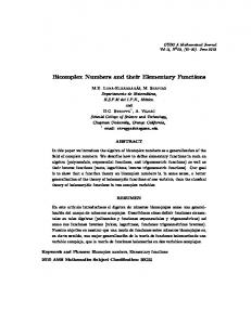
!��� "��#� �� ��� $�� �� � �� %� ��� ��� In decision diagrams based on the Shannon expansion, function values can be obtained by traversing the decision diagrams from the root node to a terminal node [9, 10]. In EVBDDs and EVMDDs, function values can be obtained as the sum of the weights for traversed edges. Fig. 4 shows the function generator based on EVMDD. It consists of a memory to store an EVMDD, an address computation circuit to traverse an EVMDD, and an adder to compute sum of edge weights. Note that for readability of the figures, registers, circuits for initialization, and some signals are omitted from Fig. 4. In Fig. 4 (a), the memory for EVMDD stores data for edges in an EVMDD. Data for an edge consist of a pointer to the next node, data for next variable of the next node,
Table 4. Memory data for the function generator for 2-bit precision 2-D norm function. Edge Shift Mask data Address of Edge address data (binary) next node weight 0 1 001 8 0 1 1 001 8 2 2 0 000 0 1 3 1 001 8 2 4 0 000 0 2 5 1 001 8 3 6 0 000 0 3 7 0 000 0 4 8 0 000 0 0 9 0 000 0 1 Initial values Shift data: 0 Mask data: 111 Address of node: 0 Edge weight: 0
and an edge weight. From the memory, a pointer to the next node and data for next variable are read and fed to the address computation circuit. And, an edge weight is fed to the adder. The address computation circuit produces an address of the next edge, from an address of node and a value of the input variable. Fig. 4 (b) shows the address computation circuit. Data for next variable consist of shift data and mask data. A value of the corresponding input variable is retrieved by the left shifter and the AND gates. And, the value is added to the address of next node to generate the edge address. Example 6 Table 4 shows memory data and initial values for the function generator produced from the EVMDD in Fig. 3 (d). This example shows how to compute the function value for X �10�2 and Y �10�2 using Table 4. First, the address computation circuit produces an edge address from the initial values. Since the initial shift data is 0, the bitwise AND of the most significant 3 bits of input variable �x1 x0 y1 �2 �101�2 and the initial mask data �111�2 is computed to produce �101�2. Adding the initial address of node 0 to the result of bitwise AND yields the first edge address �101�2 5. Next, data for the address 5 are read from the memory and fed to the address computation circuit and the adder. The adder obtains the sum of the edge weight 3 given by the memory and the initial edge weight 0. In the address computation circuit, the value of input variable is �x0 y1 y0 �2 �010�2, which is shifted to the 1-bit left, and the bitwise AND is performed with the mask data �001�2 . Adding the result of bitwise AND 0 to the address of node 8 yields the second edge address 8. Since in data for the address 8, the mask data 0 means arrival at the terminal node, adding the edge weight 0 to the previous sum of edge weights 3 yields the function value 3. (End of Example) Since the circuit shown in Fig. 4 just traverses an EVMDD and computes sum of edge weights, it can eval-
uate both one- and two-variable functions with the same architecture.
!� � ����� �� #�� $�� �� � �� %� ����
��� &�� � ������ For given elementary function, its domain, and precision, we can systematically design the circuit in Fig. 4. First, convert a given elementary function into an n-bit precision integer-valued function, next represent the integer-valued function using an EVMDD, and finally generate HDL code for the circuit in Fig. 4 from the EVMDD. Since our function generator directly realizes the function table, it is more accurate than the existing function generators using polynomial approximation [5, 14, 20, 25, 26]. To generate memory data like Table 4, we first assign an address to each edge in an EVMDD. For each non-terminal node, we assign addresses to edges in ascending order from 0-edge. Thus, addresses assigned to 0-edges correspond to addresses of non-terminal nodes. Next, we generate shift data and mask data of each edge. For an EVMDD for f �Xu Xu 1 � � � X1 �, shift data and mask data of an edge are computed as follows: u 1
shift data
∑ kj
mask data
2ki � 1
j i
bit size for mask
max �k j �
1� j �u
where the edge points to a node representing Xi , variable order of the EVMDD is Xu Xu 1 � � � X1 from the root, and k j X j � j 1 2 � � � u �. Memory size and delay time of our function generator depend largely on memory size and path length of EVMDD. Therefore, the memory minimization algorithm and the APL minimization algorithm for MDDs [17, 18] are useful to produce fast and compact function generators.
5. Conclusion and Comments This paper has introduced a new class of integer-valued functions, called an l-restricted Mp-monotone increasing function. It has also derived an upper bound on the number of nodes in an EVBDD to represent the function. EVBDDs represent l-restricted Mp-monotone increasing functions or their linear transformations more compactly than MTBDDs and BMDs when p is small. This paper has also presented a design method for function generators based on EVMDDs. With EVMDDs, we can realize accurate, fast, and compact function generators for two-variable elementary functions. In FPGA implementations for two-variable elementary functions, we confirmed that EVMDD-based function generators require, on the average, only 37% of the delay time and 62% of the memory size needed for EVBDD-based function generators.
Our future works include deriving lower bounds on the number of nodes in decision diagrams, and designing faster and more compact function generators.
Acknowledgments
[13] Y-T. Lai, M. Pedram, and S. B. Vrudhula, “EVBDD-based algorithms for linear integer programming, spectral transformation and functional decomposition,” IEEE Trans. Comput.-Aided Des. Integr. Circuits Syst., Vol. 13, No. 8, pp. 959–975, Aug. 1994. [14] D.-U. Lee, W. Luk, J. Villasenor, and P. Y. K. Cheung, “Hierarchical segmentation schemes for function evaluation,” Proc. of the IEEE Conf. on Field-Programmable Technology, Tokyo, Japan, pp. 92– 99, Dec. 2003.
This research is partly supported by the Grant in Aid for Scientific Research of the Japan Society for the Promotion of Science (JSPS), funds from Ministry of Education, Culture, Sports, Science, and Technology (MEXT) via Knowledge Cluster Initiative, the MEXT Grant-in-Aid for Young Scientists (B), and Hiroshima City University Grant for Special Academic Research (General Studies).
[17] S. Nagayama and T. Sasao, “Compact representations of logic functions using heterogeneous MDDs,” IEICE Trans. on Fundamentals, Vol. E86-A, No. 12, pp. 3168–3175, Dec. 2003.
References
[18] S. Nagayama and T. Sasao, “On the optimization of heterogeneous MDDs,” IEEE Trans. on CAD, Vol. 24, No. 11, pp. 1645–1659, Nov. 2005.
[1] H. Anton, Multivariable Calculus, John Wiley & Sons, Inc., 1995. [2] R. E. Bryant, “Graph-based algorithms for boolean function manipulation,” IEEE Trans. Comput., Vol. C-35, No. 8, pp. 677–691, Aug. 1986. [3] R. E. Bryant and Y-A. Chen, “Verification of arithmetic circuits with binary moment diagrams,” Design Automation Conference, pp. 535–541, 1995. [4] E. M. Clarke, K. L. McMillan, X. Zhao, M. Fujita, and J. Yang, “Spectral transforms for large Boolean functions with applications to technology mapping,” Proc. of 30th ACM/IEEE Design Automation Conference, pp. 54–60, June 1993. [5] J. Detrey and F. de Dinechin, “Table-based polynomials for fast hardware function evaluation,” 16th IEEE Inter. Conf. on Application-Specific Systems, Architectures, and Processors (ASAP’05), pp. 328–333, 2005. [6] R. Drechsler and B. Becker, Binary Decision Diagrams: Theory and Implementation, Kluwer Academic Publishers, 1998. [7] R. Gutierrez and J. Valls, “Implementation on FPGA of a LUT based atan�y�x� operator suitable for synchronization algorithms,” Proc. of the IEEE Conf. on Field Programmable Logic and Applizations, pp. 472–475, Aug. 2007. [8] Z. Huang and M. D. Ercegovac, “FPGA implementation of pipelined on-line scheme for 3-D vector normalization,” Proc. of the 9th Annual IEEE Symp. on Field-Programmable Custom Computing Machines (FCCM’01), pp. 61–70, Apr. 2001. [9] Y. Iguchi, T. Sasao, M. Matsuura, and A. Iseno, “A hardware simulation engine based on decision diagrams,” Asia and South Pacific Design Automation Conference (ASP-DAC’2000), pp. 73–76, Yokohama, Japan, Jan. 2000. [10] Y. Iguchi, T. Sasao, and M. Matsuura, “Evaluation of multipleoutput logic functions using decision diagrams,” Asia and South Pacific Design Automation Conference (ASP-DAC’2003), pp. 312– 315, Kitakyushu, Japan, Jan. 2003. [11] T. Kam, T. Villa, R. K. Brayton, and A. L. SangiovanniVincentelli, “Multi-valued decision diagrams: Theory and applications,” Multiple-Valued Logic: An International Journal, Vol. 4, No. 1-2, pp. 9–62, 1998. [12] Y-T. Lai and S. Sastry, “Edge-valued binary decision diagrams for multi-level hierarchical verification,” Proc. of 29th ACM/IEEE Design Automation Conference, pp. 608–613, 1992.
[15] C. Meinel and T. Theobald, Algorithms and Data Structures in VLSI Design: OBDD – Foundations and Applications, Springer, 1998. [16] J.-M. Muller, Elementary Function: Algorithms and Implementation, Birkhauser Boston, Inc., Secaucus, NJ, 1997.
[19] S. Nagayama and T. Sasao, “Representations of elementary functions using edge-valued MDDs,” 37th International Symposium on Multiple-Valued Logic, Oslo, Norway, May 13-16, 2007. [20] J.-A. Pi˜neiro, S. F. Oberman, J.-M. Muller, and J. D. Bruguera, “High-speed function approximation using a minimax quadratic interpolator,” IEEE Trans. on Comp., Vol. 54, No. 3, pp. 304–318, Mar. 2005. [21] R. Rudell, “Dynamic variable ordering for ordered binary decision diagrams,” International Conference on Computer-Aided Design (ICCAD’93), pp. 42–47, Nov. 1993. [22] T. Sasao and M. Fujita (eds.), Representations of Discrete Functions, Kluwer Academic Publishers, 1996. [23] T. Sasao, Switching Theory for Logic Synthesis, Kluwer Academic Publishers, 1999. [24] T. Sasao and S. Nagayama “Representations of elementary functions using binary moment diagrams,” 36th International Symposium on Multiple-Valued Logic, Singapore, May 17-20, 2006. [25] T. Sasao, S. Nagayama, and J. T. Butler, “Numerical function generators using LUT cascades,” IEEE Transactions on Computers, Vol. 56, No. 6, pp. 826–838, Jun. 2007. [26] M. J. Schulte and J. E. Stine, “Approximating elementary functions with symmetric bipartite tables,” IEEE Trans. on Comp., Vol. 48, No. 8, pp. 842–847, Aug. 1999. [27] R. Stankovic and J. Astola, Spectral Interpretation of Decision Diagrams, Springer Verlag, New York, 2003. [28] R. Stankovic and J. Astola, “Remarks on the complexity of arithmetic representations of elementary functions for circuit design,” Workshop on Applications of the Reed-Muller Expansion in Circuit Design and Representations and Methodology of Future Computing Technology, pp. 5–11, May 2007. [29] N. Takagi and S. Kuwahara, “A VLSI algorithm for computing the Euclidean norm of a 3D vector,” IEEE Transactions on Computers, Vol. 49, No. 10, pp. 1074–1082, Oct. 2000. [30] M. A. Thornton, R. Drechsler, and D. M. Miller, Spectral Techniques in VLSI CAD, Springer, 2001. [31] I. Wegener, Branching Programs and Binary Decision Diagrams: Theory and Applications, SIAM, 2000. [32] S. N. Yanushkevich, D. M. Miller, V. P. Shmerko, and R. S. Stankovic, Decision Diagram Techniques for Micro- and Nanoelectronic Design, CRC Press, Taylor & Francis Group, 2006.