Transport and Telecommunication
Vol.7, No 1, 2006
RESEARCH OF A STATISTICAL PROCESS CONTROL IN SOFTWARE ENGINEERING PROJECT Jurijs Senbergs1, Boriss Misnevs2 Transport and Telecommunication Institute Lomonosov Str.1, Riga, LV-1019, Latvia Ph: (+371)-7100650. Fax: (+371)-7100660 1 E-mail:
[email protected] 2 E-mail:
[email protected]
This paper presents some results of the “Research of a Statistical Process Control in Software Engineering Project”, which was performed in Transport and Telecommunication Institute.The purpose of the research was evaluation of stability of Software Engineering processes of the Organization.
Keywords: software measurement, process management and improvement, statistical control
The research was based on the information of an IT related division of a large state company. The subject of the research was internal software product development project started in 1997 and based on DBMS Oracle platform. Data model has a very complex structure and is continuously modified. The objects of research were software engineering process maturity characteristics. The main problem was that the organization was not informed about real software engineering process attributes, which may be used for problem solving. Before the research actuality was started a lot of findings over Internet related to the research topic were investigated. For example, more than 120 conference reports on “Software Measurement” were reviewed. We used the following two main definitions of base process characteristics – stable process and capable process. Stable process — the underlying distributions of its measurable characteristics are consistent over time, and the results are predictable within determined limits. Capable process – it is stable, meeting specifications process. There were the following four research tasks: 1) Developed process stability hypotheses proof / declining; 2) Out-of-control situation detection, cause understanding and prevention; 3) Control limits definition for further process stability investigation; 4) Process capability definition. Research process was separated into three sub activities. They are as follows: Collect and retain data, Analyze data and Act on results. Data from two last years containing 422 defect reports, 108 change requests with related process information were collected for the analyses. As an analyses tool the Control chart was utilized. During this phase control limits and out-of-control situations were detected. The last phase was related to the process capability definition. Every detected out-of-control situation was checked regarding possible out-of-control situation to refrain from repetition.
Six processes with two main characteristics (number and time) were selected for the stability research. The research was using variable data from continues measurements; the appropriate Xband and R control charts were selected. The Shewhart or 3 sigma deviation control limits were used for limit control management. The centre line and control limits were calculated and placed into charts. Values were grouped into sub groups. For the first three processes weeks, and one group – by months, grouped the data. For all other processes the sub group is a quarter. After that 70
Proceedings of the 5th International Conference RelStat’05
Part 1
populated values were compared with calculated limit values. If a populated value is placed upper or lower of the centreline, but within control limits, this means that the process was stable during the period of measurements. If any measuring value is out of the limit it means that the process is not stable. In this case we have to assess the cause of the deviation and fix it to prevent the case repetition. (If the fix is successful we have to introduce this improvement into the process as an integral part of it). The procedure for X-bar and R chart limit calculation is the following: 1. Calculate average value X and variation R for each k sub group; 2. Calculate common average value X , calculating average value X from k sub group average value; 3. Calculate common average value X , calculating average value X from k sub group average value; 4. Calculate deviation average value R , calculating each k sub groups deviation R; 5. Centre line for the chart is X , centre line for the R chart is R . Select from the table values of A2, D3 and D4, which are in accordance with the sub group size n; 6. Multiply A2 to R receiving A2 R . Add common average X value to A2 R to get the upper control limit – UCLx; 7. Subtract from common average X value A2 R to get the lower control limit LCLx; 8. Multiply D4 and R to get the upper control limit to R chart. Multiply D3 and R to get the lower control limit to R chart.
Constants for Computing Control Limits for X-Bar and R Charts from [1]
Two of four General Electric described tests were used for the purpose of unstable and out-ofcontrol situations assessing. They were the most effective from the author’s point of view. They are the following: 1. One point is out of 3 sigma limits; 2. At least two points from three consecutive points deviate to one and the same side for more that 2-sigma distance from the centreline. 71
Transport and Telecommunication
Vol.7, No 1, 2006
The following processes were selected for the stability research as processes directly connected to the customer and the developer: Defect reports management process: Critical defects detection, Critical defects fixing, Change requests management process: Change request application, Change approval, Change request closing, and Change request implementation. First example is critical defects detection process. The process was assessed using the approach described earlier. The question was “Is the Process stabile or not?” As the main process characteristic was used number of defects. Analyzed data covers 2003 and 2004 years critical defect management process. Data was grouped on the weekly base. Control chart represents one group as one point per months. Control chart limits were detected using the same approach as was discussed earlier. Out-of-control cases were not discovered. There are no 2 sequential points deviating 2-sigma from the centreline. This means that the critical defect management process is stable and is in accordance with process quality requirements. From the chart we may find that we have 3.2 defects per week as an average value. All R charts are in control limits. Second example is critical defects fixing process (time for fixing). The process stability assessment using the discussed approach was performed and characteristics defined. The question is “May we consider the process as stable?” The defect fixing statistics for 2003 and 2004 years were used as the data for the analysis. Data were divided into weekly sub groups. But 72
Proceedings of the 5th International Conference RelStat’05
Part 1
in control charts one point is one month. Control limit charts were created using the method mentioned earlier. Because one point is out of control limit the process was assessed as out of control. Because of X-bar chart standard deviation sigma X is as standard deviation from individual values it is divided to
n , where n is sub group size (measurements number). That upper control limit
for capability histogram UCLx is equal to X + 3sigma X . And lower control limit for capability histogram LCLx is equal to X − 3sigma X . To confirm the process stability need also to put capability histogram into specification limit. Relation between capability histogram and specification limits reflects the process capability. Optimal value or target is calculated as average from upper (USL) and lower (LSL) specification limits LSL +
USL − LSL USL − LSL . Specification tolerance is equal to . 2 sigma X
Distance to the nearest specification is equal to
USL − X . sigma X
It is clear from capability histogram that the process values distribution is approximately within control limits. Lower specification level (LSL) is equal to 1 and upper specification level (USL) is equal to 11. The distribution must be symmetric and the target (or optimal value) is equal to 6. Then the specification tolerance is equal to 10 fixed defects per week and a specification tolerance sigma item is equal to 2.79. The distance to the nearest specification is equal to 2.11. From the received results we can see that the specification tolerance sigma item critical defects detection process is equal to 2.79 and does not exceeds six sigma items. This means that only 47% of all values are within the specification limits, but the process is stabile. This also means that the process is stabile, but is not enough capable and repeatable out-of-range values often exceed the specification limits. To do the process more capable it is possible to perform the following activities: prevent the process variability, change the process average or decrease the specification requirements.
Capability histogram for the process of critical defects detection
For example, if for the critical defect fixing process deviation is decreased for the level ~3 than upper control limit constricts to ~9. In this case control limit is placed into specification limit and the process capability is increased to 7. This means that the process is in accordance to the specification. In this case distance from upper control limit to lower control limit is the field of refinement. Values, which are outside of the control limits, are the process defects, which can be removed and, if this is done before they overcome upper specification limit, means that client will never see them. In other words the process will be stabilized timely and specification requirements will be always implemented. 73
Transport and Telecommunication
Vol.7, No 1, 2006
Capability histogram for the defect correction process after its refinement
Although it is possible to refine the process further. From the capability histogram we can state that the process is not centred enough. This means that the DNS index is not high. Through the moving average value to the specification average value will guarantee good DNS index. For example, if critical defects fixing process average value is near to specification average value from 4 to 5 (distance will be reduced from 2 to 1; DNS will be increased from 4.2 to 4.5. Both DNS will overcome 3 sigma items, but the process becomes more centred). During the research it was concluded that for further analyses we need to investigate individual values, or XmR charts. Because the X-bar charts using average values do not always reflect all out-ofcontrol situations. For example, for the change request implementation process in X-bar charts populated values were within the control limits, but in the process capability assessment histograms it seems that separate values are out of the upper control limit.
Capability histogram for change request implementation process
During the research the following statements were proved: 1) Two from the six investigated processes are stable and may be used for the future situation forecasting; 74
Proceedings of the 5th International Conference RelStat’05
Part 1
2) For four processes out-of-control values are detected, causes are detected un control limits are recalculated; 3) Out-of-control situation in the first process affects other process and causes out-of-control situation for the second process; 4) Defined control limits may me used for further process stability investigation; 5) The Organization Process capability is defined; 6) More deep process analyses may be done only investigating individual values of the process characteristics (e.g. using XmR charts).
References [1] Florac W., Park R., Carleton A. Practical Software Measurement: Measuring for Process Management and Improvement, CMU/SEI-97-HB-003, April 1997, 246 p. [2] David N. Card “Sorting out Six Sigma and the CMM”, IEEE Software JNL, May 2000, pp. 11-13. [3] Caivano D. Continuous Software Process Improvement through Statistical Process Control. In: Ninth European Conference on Software Maintenance and Reengineering (CSMR'05), March 2005, pp. 288-293. [4] Eickelmann N., Anant A. Statistical Process Control: What You Don’t Measure Can Hurt You! IEEE Software JNL, March 2003, pp. 49-51. [5] Florac W., Carleton A, Barnard J. Statistical Process Control: Analyzing a Space Shuttle Onboard Software Process, IEEE Software JNL, July 2000, pp. 97-106. [6] Misnevs B., Daineko D. Developing a New Testing Model, Transport and Telecommunication, Vol.3, No 1, 2002, pp. 26-33.
75