for a parallel computer will schedule the waiting jobs. .... To find the best parameters for the instance based learning techniques, we search over traces from.
Resource Selection Using Execution and Queue Wait Time Predictions Warren Smith Parkson Wong Computer Sciences Corporation NASA Ames Research Center Moffett Field, CA 94035 {wwsmith, parkson}@nas.nasa.gov
NAS Technical Report Number: NAS-02-003 July 2002 Abstract Computational grids provide users with many possible places to execute their applications. We wish to help users select where to run their applications by providing predictions of the execution times of applications on space shared parallel computers and predictions of when scheduling systems for such parallel computers will start applications. Our predictions are based on instance based learning techniques and simulations of scheduling algorithms. We find that our execution time prediction techniques have an average error of 37 percent of the execution times for trace data recorded from SGI Origins at NASA Ames Research Center and that this error is 67 percent lower than the error of user estimates. We also find that the error when predicting how long applications will wait in scheduling queues is 95 percent of mean queue wait times when using our execution time predictions and this is 57 percent lower than if we use user execution time estimates.
1. Introduction The existence of computational grids allows users to easily execute their applications on a variety of different computer systems. The obvious question users have each time they wish to run an application is which computer system should they use? Many factors go into making this decision: The computer systems that the user has access to, the user’s remaining allocations on these systems, the cost of using different systems, the location of data sets for the experiment, how long the application will execute on different computers, when the application will start executing, and so on. In this work, we address the problems of predicting how long an application will execute on different computer systems and predicting when scheduling systems for such computers will start an application. With this information, we can calculate when an application will complete executing and we can use these predictions to suggest which computer system to use for an application. The exact problems we address are predicting how long parallel applications will execute on space shared parallel computers and predicting how long these applications will wait in scheduling queues before they are given access to resources. We predict the execution time of applications using an historical database and instance-based learning techniques. Each data point in the database is one application execution, or job, that has run in the past. When an execution time estimate needs to be calculated, instance-based learning techniques find historical jobs that are similar to the job being estimated, and derive a prediction from those historical jobs.
1
We find that our execution time prediction technique has an average error of 37 percent of the average execution times of six months of jobs submitted to three SGI Origins located at the NAS division at the NASA Ames Research Center. We also compared the performance of our prediction technique to three other techniques that have been developed. We find that our technique currently has a 7 percent lower error than the best of these three techniques for jobs executed on four supercomputers at three different centers. Our approach to predicting when a job will execute on a parallel computer is to predict the execution times of all of the jobs running and waiting to run and then simulate how the scheduler for a parallel computer will schedule the waiting jobs. This simulation gives us an estimated start time for each job that is waiting to execute. If we predict the start time of every job in one of our NASA Ames traces as it is submitted, we find that the average error of this approach is 95 percent of the average scheduling queue wait time when using First-Come First-Served scheduling but this is 57 percent better than if we use user execution time estimates instead of our execution time predictions.
2. Execution Time Prediction We predict the execution time of applications using instance based learning techniques that are also called locally weighted learning techniques [2, 10]. In this type of technique, a database of experiences, called an experience base, is maintained and used to make predictions. Each experience consists of input and output features. Input features describe the conditions under which an experience was observed and the output features describe what happened under those conditions. Each feature typically consists of a name and a value where the value is of a simple type such as integer, floating point number, or string. When a prediction is to be performed a query point consisting of input features is presented to the experience base. The data points in the experience base are examined to determine how relevant they are to the query. Relevance is determined using the distance between an experience and the query. There are a variety of distance functions that can be used [13] and we have chosen to use the Heterogeneous Euclidean Overlap Metric. This distance function can be used on features that are linear (numbers) or nominal (strings). We require support for nominal values because important features such as the names of executables, users, and queues are nominal. The distance between experience x and experience y is defined as:
D ( x, y ) =
�d f
( x, y )2
f
Where f is a certain feature and d f ( x, y ) is the per-feature distance. This is very similar to the Euclidean distance, except that to support nominal values, the following per-feature distance is used: �
1,
�
if x f or y f is unknown, else
d f ( x, y ) = � overlap f ( x, y ), if f is nominal, else � �
rn _ diff f (x, y )
With the following definitions:
0, if x f = y f �
overlap f ( x, y ) = �
rn _ diff f =
1, otherwise
�
2
xf − yf max f − min f
The per-feature distance between two nominal values is 0 if they are the same and 1 otherwise. For linear values, the distance is their difference scaled by the range of values for feature f in the experience base. This approximately scales the distance to be between 0 and 1. As a further refinement, we perform feature scaling to stretch the experience space and have it be more important that certain features are similar than others. To accomplish this, we add feature weights, w f , to our distance function:
D ( x, y ) = '
� wf d f
(x, y )2
f
Once we know the distance between experiences and a query point, the next question to be addressed is how we calculate estimates for the output features of the query point. For linear output features, such as execution time, our approach is to use a distance-weighted average of the output features of the experiences to form an estimate. We use kernel regression to form estimates and following kernel function to form the estimate E for output feature f of a query point q:
E f (q ) =
�K
(D(q, e))V f (e )
e
�K
(D(q, e ))
e
where K is the kernel function, D is the distance function described previously, e is an experience in the experience base, and V f (e ) is the value for feature f of experience e. The kernel function is used to weight the values of the features in the experience base based on distance. The kernel function should approach a constant value as the distance goes to 0 and should approach 0 as the distance goes to infinity. This results in experiences closer to the query point having a larger contribution to what the estimate will be. There are a wide variety of kernel functions that can be used. We have chosen to use a simple Gaussian function. Further, we have included a kernel weight so that we can compact or stretch the kernel to give lower or higher weights to experiences that are farther away. The resulting kernel function is:
K (d ) = e
�
−� �
d k
2 �
� �
In the previous discussion, we have described the kernel width and feature weight parameters that need to be selected. Two other parameters we need values for are the maximum experience base size and the number of nearest neighbors (experiences) to use when making an estimate. Specifying the number of nearest neighbors to use allows us to decrease the amount of time it takes to calculate an estimate, but we do not want this to adversely impact estimation performance. Our approach to determine the best values for these parameters is to perform a genetic algorithm search [7] to try different values and attempt to minimize the prediction error. In our approach, a scheduling job can be an experience or a query. When a job finishes executing, it becomes an experience that is inserted into the experience base. This experience consists of input features such as the user who submitted the job, the application that was executed, the number of CPUs requested, and so on. The execution time of the job is the only output feature of the experience. When a user wants a prediction for how long a job will execute, the job is turned into a query that contains the input features just described. An estimate for the execution time output feature of the query is made using the techniques we have described above.
3
2.1. Performance We evaluate the performance of our execution time prediction technique using trace data recorded from three SGI Origins located at the NASA Ames Research Center. The traces were recorded during 2001 from the system lomax, that had 496 CPUs available to users, steger that had 248 CPUs available, and hopper that had 60 CPUs available. For each job, the relevant information in the traces is the user who submitted the job, the name of the job, the number of CPUs requested, the amount of wall clock time the CPUs were requested for, the amount of wall clock time actually used, and when the job was submitted. To find the best parameters for the instance based learning techniques, we search over traces from May and June of 2001. In all cases, we initialized our experience base with the jobs that completed in May. For steger and hopper, we predict all of the jobs that were submitted in June and inserted all of the jobs that finished in June. We use the accuracy of these predictions to evaluate the parameters selected. Lomax had a large number of jobs submitted in June so we only used the first week of data from June and evaluated the parameters using the accuracy of the predictions in this week of data. The best parameters we found are shown in Table 1. The two obvious trends are that the number of nearest neighbors is relatively small and the feature weight for the number of CPUs is relatively high. Table 1. The best instance based learning parameters found by our genetic algorithm searches. Parameter Nearest neighbors Experience base size Kernel width Job name weight User name weight Number of CPUs weight Requested time weight Current time weight
Workload Lomax Steger Hopper 25 8 7 1200 1161 8486 12.0 36.5 18.0 65.7 83.1 31.4 4.9 57.4 99.2 67.0 77.7 79.6 66.0 17.6 101.7 54.0 74.1 39.9
After we find the parameters to use for the instance based learning techniques, we evaluate the accuracy of these configurations using trace data from July through December of 2001. We use this approach to accurately reflect how searches would be performed and used in reality. Table 2 shows the accuracy of our predictions along with the accuracy of user estimates and the mean run times of the applications in the workloads. The table shows the mean error of our predictions is between 36 and 39 percent of the mean run time while the error of the user estimates is between 87 and 149 percent of the mean run time. One fact to note about the user estimates are that users are encouraged to over estimate their execution time because their applications are terminated if they use more time than they estimate. Table 2. Execution time prediction error on traces recorded during the last 6 months of 2001. System lomax steger hopper
Mean Error (minutes) 36.27 22.45 22.16
Mean Error of User Estimate (minutes) 86.00 61.31 84.56
4
Mean Run Time (minutes) 98.80 63.04 56.91
2.2. Previous Work There have been several efforts to attempt to predict the execution time of serial and parallel applications. There have been many efforts to predict the execution time of serial applications on loaded computer systems [3, 4, 8, 14]. Kapadia used instance based learning techniques, the same class of techniques we use, to also predict serial applications on loaded computer systems [9]. Another effort estimated the performance of components of distributed applications [11]. Several researchers, including one of the authors, have addressed the problem of predicting the execution time of parallel applications on space shared parallel computers by categorizing completed applications and calculating a prediction from the completed applications in the category the application to predict falls in [5, 6, 12]. In [12] it was shown that the prediction technique developed by Smith has lower prediction error than the approaches of Downey and Gibbons. Table 3 shows a comparison of Smith’s technique and our technique using trace data from 3 months of data from IBM SP that was at Argonne National Laboratory during 1996, 12 months of data from the IBM SP that was at the Cornell Theory Center in 1996, and two 12 month traces from the Intel Paragon that was at the San Diego Supercomputing Center in 1995 and 1996. The table shows that at the current time, our instance based learning technique has 7 percent lower prediction error than the approach of Smith. Table 3. A comparison of our execution time prediction technique to those of Smith. Workload ANL CTC SDSC95 SDSC96
Our Mean Error (minutes) 41.52 105.71 50.81 59.24
Mean Error for Smith (minutes) 38.48 106.73 59.65 74.56
Mean Error of User Estimate (minutes) 104.35 222.71 N/A N/A
Mean Run Time (minutes) 97.08 182.49 108.16 166.85
3. Start Time Prediction Our approach to predicting when applications submitted to scheduling systems will begin executing is relatively simple: we perform a simulation of the scheduling algorithm which results in estimated start times for each of the applications waiting in the queue. This simulation is performed using predictions of the run times of the applications because the actual run times are not known. We evaluate the performance of this technique using six months of trace data from July through December of 2001 recorded from the SGI Origins lomax, steger, and hopper. When using our prediction techniques, we first load the execution experiences from June of 2001 into the experience base and then simulate the following six months of data. We use the execution time prediction configuration that we found using our searches of Section 2.1. So far, we have only had time to evaluate this approach using the First-Come First-Served scheduling algorithm and the trace data from hopper. We will evaluate other scheduling algorithms, such as backfill, using trace data from lomax, steger, and hopper for the final version of this paper. Table 4 shows the prediction error of our technique when our run time predictions are used and when the user estimates are used. We do not show that when the exact execution times of the applications are known, we can exactly predict how long each application will wait in the queue. The data shows that if we use the estimates of run times made by users, the error is 222 percent of 5
the mean wait time. If our run time estimates are used, the error is only 95 percent of the mean wait time. This is an improvement of 57 percent. We expect to reduce our start time prediction error for the final version of this paper by optimizing our instance based learning parameters for the execution time predictions made here instead of the ones made in Section 2.1. Table 4. Start time prediction error for trace data from the last six months of data in 2001 and First-Come First-Served scheduling. Workload
Hopper
Mean Error using User Run Time Estimate (minutes) 124.48
Mean Error using Predicted Run Time (minutes) 53.09
Mean Wait Time (minutes) 56.03
4. Implementation We have implemented a prototype service to provide predictions using our techniques. This service can be used to provide execution time predictions, start time predictions, completion time predictions (start time prediction plus the execution time prediction), and suggestions of which machine to use. The suggested machine is the one that will complete an application earliest. We have deployed this prototype service for use in the SGI Origin cluster at Ames that consists of the machines lomax, steger, and hopper. These systems are all scheduled using PBS[1] and the architecture of this service is shown in Figure 1. The prediction service is executing on a system at Ames and can be accessed from client command line programs on remote computer systems. The command line programs allow users to ask for the predictions and suggestions described above. These programs can be run on jobs already submitted to the PBS schedulers or on PBS scripts that are about to be submitted. To accomplish this, the system has been programmed to be able to parse PBS scripts to pull out job information, to monitor the jobs that exist in PBS scheduling systems, and to simulate the scheduling algorithms used on our Origins. We have just begun to evaluate this implementation and do not have performance data to present at this time. Prediction Server Prediction Client Start and Completion Time Predictor Command Line Programs
Prediction Client Interface
Prediction Service Interface
PBS Scheduling Simulator Execution Time Predictor
PBS Script Parser
PBS Monitor
Experience Base PBS Monitor
Figure 1. Architecture of our prototype prediction service.
5. Conclusions and Future Work This paper presents a technique to predict the execution times of parallel applications when run on space shared parallel computers and a technique to predict how long such applications will 6
wait in scheduling queues before they are allocated resources. These predictions allow us to predict the completion time of applications that is a very useful piece of information for users that are trying to select a computer system in a computational grid. We find that our execution time prediction technique has an average error of 37 percent of the average execution times on trace data recorded from three Origins at NASA Ames Research Center. We also find that the average start time prediction error 95 percent of the average queue wait time when using First-Come First-Served scheduling but this is 57 percent better than if we use user execution time estimates instead of our execution time predictions. For the final version of this paper, we will perform more extensive searches to improve our execution time prediction accuracy and perform more analysis of our data. In the future we will also continue to improve the performance of our instance based learning techniques. In addition to investigating more advanced instance based learning techniques, we will examine other improvements such as allowing users to specify application-specific features. We will also modify the design of the prediction service presented in Section 4 so that it will operate in a full computational grid, not just at a single site.
References [1] [2] [3]
[4] [5] [6] [7] [8]
[9]
[10] [11]
[12] [13] [14]
"The Portable Batch System," http://www.pbspro.com. C. Atkeson, A. Moore, and S. Schaal, "Locally Weighted Learning," Artificial Intelligence Review, vol. 11, pp. 11-73, 1997. M. Devarakonda and R. Iyer, "Predictability of Process Resource Usage: A Measurement-Based Study on UNIX," IEEE Transactions on Software Engineering, vol. 15, pp. 1579-1586, 1989. P. Dinda, "Online Prediction of the Running Time of Tasks." In Proceedings of the The 10th IEEE International Symposium on High Performance Distributed Computing, 2001. A. Downey, "Predicting Queue Times on Space-Sharing Parallel Computers." In Proceedings of the 11th International Parallel Processing Symposium, 1997. R. Gibbons, "A Historical Application Profiler for Use by Parallel Schedulers," Lecture Notes on Computer Science, vol. 1297, pp. 58-75, 1997. D. Goldberg, Genetic Algorithms in Search, Optimization, and Machine Learning: Addison-Wesley, 1989. M. Iverson, F. Ozguner, and L. Potter, "Statistical Prediction of Task Execution Times Through Analytical Benchmarking for Scheduling in a Heterogeneous Environment." In Proceedings of the IPPS/SPDP'99 Heterogeneous Computing Workshop, 1999. N. Kapadia, J. Fortes, and C. Brodley, "Predictive Application Performance Modeling in a Computational Grid Environment." In Proceedings of the 8th IEEE International Symposium on High Performance Distributed Computing, 1999. J. Schneider and A. Moore, "A Locally Weighted Learning Tutorial using Vizier 1.0," Robitics Institute, Carnegie Mellon University CMU-RI-TR-00-18, Febuary 2000. J. Schopf and F. Berman, "Performance Prediction in Production Environments." In Proceedings of the 12th International Parallel Processing Symposium and the 9th Symposium on Parallel and Distributed Processing, 1998. W. Smith, I. Foster, and V. Taylor, "Predicting Application Run Times Using Historical Information," Lecture Notes on Computer Science, vol. 1459, pp. 122-142, 1998. D. R. Wilson and T. R. Martinez, "Improved Heterogeneous Distance Functions," Journal of Artificial Intelligence Research, vol. 6, pp. 1-34, 1997. R. Wolski, N. Spring, and J. Hayes, "Predicting the CPU Availability of Time-Shared Unix Systems." In Proceedings of the 8th IEEE International Symposium on High Performance Distributed Computing, 1999.
7