Retinotopic Axis Specificity and Selective ... - Semantic Scholar

The Journal of Neuroscience, February 23, 2005 • 25(8):2117–2131 • 2117

Behavioral/Systems/Cognitive

Retinotopic Axis Specificity and Selective Clustering of Feedback Projections from V2 to V1 in the Owl Monkey Amir Shmuel,1,2 Maria Korman,1 Anna Sterkin,1 Michal Harel,1 Shimon Ullman,2 Rafael Malach,1* and Amiram Grinvald1* Departments of 1Neurobiology and 2Computer Science and Applied Mathematics, The Weizmann Institute of Science, 76100 Rehovot, Israel

Cortical maps and feedback connections are ubiquitous features of the visual cerebral cortex. The role of the feedback connections, however, is unclear. This study was aimed at revealing possible organizational relationships between the feedback projections from area V2 and the functional maps of orientation and retinotopy in area V1. Optical imaging of intrinsic signals was combined with cytochrome oxidase histochemistry and connectional anatomy in owl monkeys. Tracer injections were administered at orientation-selective domains in regions of pale and thick cytochrome oxidase stripes adjacent to the border between these stripes. The feedback projections from V2 were found to be more diffuse than the intrinsic horizontal connections within V1, but they nevertheless demonstrated clustering. The clusters of feedback axons projected preferentially to interblob cytochrome oxidase regions. The distribution of preferred orientations of the recipient domains in V1 was broad but appeared biased toward values similar to the preferred orientation of the projecting cells in V2. The global spatial distribution of the feedback projections in V1 was anisotropic. The major axis of anisotropy was systematically parallel to a retinotopic axis in V1 corresponding to the preferred orientation of the cells of origin in V2. We conclude that the feedback connections from V2 to V1 might play a role in enhancing the response in V1 to collinear contour elements. Key words: monkey; cortex; cerebral cortex; vision; visual cortex; striate cortex; V1; V2; feedback connections; cortical maps; orientation; orientation map; retinotopic map; retinotopy; cytochrome oxidase

Introduction Feedback connections (FbkCon) constitute a subset of corticocortical fibers, defined by specific cortical layers of cell origin and axonal termination (Rockland and Pandya, 1979; Maunsell and Van Essen, 1983; Felleman and Van Essen, 1991). This study aimed at establishing whether an organizational relationship exists between the feedback projections (FbkPrj) from V2 and the maps for orientation and retinotopy in V1. Previous studies demonstrated a nonrandom relationship between the intrinsic horizontal connections (HrzCon) (Fisken et al., 1975; Creutzfeldt et al., 1977; Gilbert and Wiesel, 1979; Rockland and Lund, 1982) and the functional maps within V1. The HrzCon selectively interconnect the systems of cytochrome oxidase (CO)-stained blobs or interblobs (Livingstone and Hubel, 1984b; Yabuta and Callaway, 1998). Clusters formed by the HrzCon preferentially interconnect columns of similar ocular dominance in macaque V1 (Malach et al., 1993; Yoshioka et al., Received Jan. 14, 2004; revised Jan. 6, 2005; accepted Jan. 7, 2005. This study was supported by grants from the Goldsmith, Glasberg, and Minerva Foundations, by the Israel Science Foundation, by M. M. Enoch (A.G., R.M., and S.U.), and by a long-term fellowship from the European Molecular Biology Organization (A.S.). We thank L. Sincich and the anonymous reviewers for their helpful comments on a previous version of this manuscript, A. Schu¨z for helpful discussions, and S. R. Smith for scientific editing. R. Eilam, S. Leytus, and D. Ettner provided excellent support. This study is dedicated to the memory of Chaipi Wijenbergen, whose innovation and support made it possible. *R.M. and A.G. contributed equally to this work. Correspondence should be addressed to Dr. Amir Shmuel, Max-Planck Institute for Biological Cybernetics, Spemannstraße 38, 72076 Tuebingen, Germany. E-mail: [email protected]. DOI:10.1523/JNEUROSCI.4137-04.2005 Copyright © 2005 Society for Neuroscience 0270-6474/05/252117-15$15.00/0

1996) and of similar preferred orientations in the cat (Gilbert and Wiesel, 1989; Kisvarday et al., 1997), tree shrew (Bosking et al., 1997), and macaque (Malach et al., 1993). The HrzCon are spatially organized in a nonrandom way in relation to the retinotopic map in V1 of the tree shrew (Fitzpatrick, 1996; Bosking et al., 1997), the cat (Schmidt et al., 1997), and the squirrel monkey (Sincich and Blasdel, 2001). In these species, labeled axons extend farther along an axis that corresponds to the preferred orientation at the injection site. Similarly, feedforward connections from layer 4 to layer 2/3 in tree shrew V1 demonstrate orientation-specific axial bias (Mooser et al., 2004). The spatial extent, orientation selectivity, and axial specificity demonstrated by the HrzCon in V1 imply that those connections might mediate geometrically specific interactions between neurons with non-overlapping classical receptive fields (RFs) (Crook et al., 2002; Stettler et al., 2002). It is unclear, however, whether the HrzCon are the exclusive neural substrates that mediate those phenomena (Angelucci et al., 2002; Crook et al., 2002). Whereas a clear relationship exists between the HrzCon and functional maps, only limited data are available for similar relationships of the connections between V1 and V2. The feedforward and the FbkCon are segregated into two separate pathways, one between blobs in V1 and thin CO stripes in V2 (Livingstone and Hubel, 1984a; Roe and Ts’o, 1999) and the other between interblobs in V1 and thick and pale CO bands in V2 (Sincich and Horton, 2002). Feedforward axon terminals in cat area 18 are confined to regions of orientation specificity similar to that of their parent cells in area 17 (Gilbert and Wiesel, 1989).

Shmuel et al. • Functional Organization of Feedback Projections

2118 • J. Neurosci., February 23, 2005 • 25(8):2117–2131

To date, no study has addressed the question of retinotopic axial specificity of the cortical FbkPrj. The possibility of orientation specificity of these projections is a matter of debate. Although Angelucci et al. (2002) predicted such specificity, Stettler et al. (2002) ruled it out. Moreover, although clustering of the FbkPrj is a prerequisite of orientation specificity, the issue of clustering is controversial. Evidence exists for both clustering (Wong-Riley, 1979a; Livingstone and Hubel, 1984a; Rockland and Virga, 1989) and diffuse projections (Rockland and Pandya, 1979; Maunsell and Van Essen, 1983; Ungerleider and Desimone, 1986). Angelucci et al. (2002) demonstrated FbkCon that terminate in clusters, whereas Stettler et al. (2002) doubted whether patchiness exists for the projections from V2 to V1. The present study aimed at investigating possible organizational relationships of the FbkPrj from V2 to the CO-dense structures and to the orientation and retinotopic maps in V1. Optical imaging of intrinsic signals (Grinvald et al., 1986) was combined with CO histochemistry and connectional anatomy in owl monkeys.a The findings indicate that these FbkCon might play a role in enhancing the response in V1 to collinear visual features. Parts of this work have been published previously in abstract form (Shmuel et al., 1998).

Materials and Methods The procedures used for preparing and maintaining the animals and for tracer injections and histology were described by Malonek et al. (1994) and Malach et al. (1993, 1994), respectively. The methods of optical imaging and analysis of functional maps were described by Shmuel and Grinvald (1996) and Bonhoeffer and Grinvald (1996). In the following, these procedures are presented in outline, whereas new methodological aspects are described in detail.

Animals Data on FbkPrj were obtained from six adult owl monkeys (Aotus nancimai) weighing between 0.8 and 1.1 kg. Data on the HrzCon within V1 were obtained from an additional monkey. A craniotomy was performed above areas V1 and V2, and the dura was removed. The imaged area extended from 1 to 16 mm away from the midline. These regions of V1 and V2 represent the lower half of the visual hemifield near the vertical meridian, between ⬃1 and ⬃15° (V1) and ⬃1 and ⬃20° (V2) from the area centralis (Allman and Kaas, 1971, 1974). A keratometer was used to fit the corneas with zero-power contact lenses. The eyes were focused on a tangent screen at a distance of 28.5–57 cm using external lenses. The areae centrales were projected onto the screen with the aid of a reversible ophthalmoscope and a fundus camera.

Visual stimuli We used a visual stimulator (STIM software; Kaare Christian, Rockefeller University, New York, NY) run on an IBM personal computer equipped with a graphics board (SGT; Number Nine Computer Corporation, Lexington, MA). The stimuli were displayed on a CRT screen in a 60 Hz non-interlaced mode. They subtended an angle of 25–50° in the visual field contralateral to the imaged hemisphere. To obtain retinotopic maps, monocular stimulation of the eye contralateral to the imaged hemisphere was used. To obtain orientation maps in V1 and V2, the monkeys were stimulated binocularly with high-contrast rectangularwave gratings with a spatial frequency of 0.5–1.0 cycles/degree and a duty cycle of 33%. The set of stimuli included four differently oriented gratings, spanning the orientation spectrum at a resolution of 45°. The gratings moved alternately in the two directions orthogonal to their orientation at a temporal frequency of 5 Hz.

a

These nocturnal simians have a rod-dominated retina and a single cone type; thus, they lack color vision. Despite these differences from diurnal primates, the CO cytoarchitecture of area V1 in owl monkeys is characterized by a mosaic of blobs and interblobs, and area V2 is characterized by a regular system of thick, pale, and thin CO stripes (Tootell et al., 1985). V1 and V2 in owl monkeys are visuotopically organized (Allman and Kaas, 1971, 1974). For a review of the visual system of owl monkeys, see Casagrande and Kaas (1994).

Functional data acquisition We used a differential video data acquisition system, IMAGER 2001 (Optical Imaging, Mountainside, NJ). Each data acquisition cycle started with an 8 s interstimulus interval, during which a stationary pattern of the stimulus was displayed. The stimulus then drifted for 2.5 s while images of the cortex were taken.

Analysis of functional maps Data were analyzed using self-written procedures in MATLAB (The MathWorks, Natick, MA). Orientation single-condition maps. To obtain an orientation singlecondition map, the mean cortical image obtained while stimulating with a specific orientation was divided by the mean “cocktail blank.” Highpass filtering was applied by subtracting the convolution of the result with an isotropic Gaussian with SD of 500 ␮m. Differential maps. Differential orientation maps were obtained by subtracting two single-condition maps corresponding to orthogonal orientations. Vectorial analysis. Four different orientation single-condition maps were summed vectorially on a pixel-by-pixel basis. The polar map presents the angle of the resulting vector by means of hue and its magnitude by brightness. Maps of SD. To estimate the pixelwise reliability of either a differential map or a polar map, we computed the corresponding map of SD across the imaging session. For consistent comparison of the mapping signalto-noise ratios across different experiments, pixelwise confidence intervals of the computed differential orientation maps were computed based on t statistics. Data from cortical locations in which the interval corresponding to a confidence coefficient of 0.95 was larger than the amplitude of differential maps were excluded from the computations of quantitative histograms.

Biotinylated dextran amine injections targeted at optically identified functional domains Functional maps were obtained from the vicinity of the V1/V2 border, which could be identified during the experiment according to the different layouts of the orientation domains: continuous in V1 versus at intervals in V2. The exact location of the border was verified after the experiment using CO histology (Fig. 1A). A clearly defined orientation-selective domain in V2 was selected for biotinylated dextran amine (BDA) injection. The center of this domain was marked on the functional map and transferred to the image of the cortical vasculature. The fine pattern of superficial blood vessels was viewed through an operating microscope and used as a reference to target a micropipette to the selected injection site. The pipette (8 –12 ␮m tip diameter) was moved using a micromanipulator (MO 103; Narishige, Tokyo, Japan) and was advanced perpendicular to the local pial surface to a cortical depth of 600 – 800 ␮m, estimated by the distance traversed after first touching the cortex. The tracer was iontophoretically ejected (tip positive).

Histology After the injections, the monkeys were maintained for at least 28 h under continuous monitoring of physiological state and level of anesthesia. They were then deeply anesthetized and perfused transcardially with PBS, followed by light fixation with 2.5% (by volume) paraformaldehyde and 0.5% glutaraldehyde in PBS containing 5% sucrose. The brains were removed, and the posterior half of the brain was flattened and postfixed. The tissue was sectioned parallel to the cortical surface at intervals of 50 ␮m (60 ␮m for monkey M1). The pattern of the superficial pial blood vessels was preserved at the uppermost section because of the care taken in flattening and sectioning of the cortical tissue. Two in every three sections were processed for BDA (Fig. 1B), using the procedure described by Malach et al. (1993) for processing biocytin. The interleaved third sections were processed for CO histochemistry (Fig. 1A), using the procedure described by Wong-Riley (1979b).

Anatomical data analysis The stained sections were viewed at low power with a Wild M5 macroscope equipped with light- and dark-field illumination, a camera lucida,


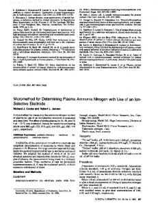
Figure 1. Tracer injection, projection patterns, and their delineation. A, V1/V2 border obtained from a CO-stained tangential section taken at a cortical depth of ⬃775 ␮m. The yellow dots that track the border were superimposed on the pattern in B after alignment. The cyan rectangle represents the extent of the dark-field image presented inB. B, Anatomical connections revealed by injection of BDA in V2. Thecoreoftheinjectedtracer(patchstainedorange-brown)andaxonalprojectionsintrinsictoV2arelocatedontheleftpartoftheimage. The axonal FbkPrj are on the right. The red and dashed white frames correspond to the magnified parts of the image presented inC/D and E,respectively.A,Anterior;P,posterior;M,medial;L,lateral.C,Bright-fieldimageoftheinjectionsite,producedathighmagnification.Note the dark saturated staining in the vicinity of the injection. D, Same as in C, after delineation of the effective-uptake zone. The red contour marks the effective tracer-uptake zone specific to the section shown here, defined using method I as the edge of the densely labeled saturatedregion.Eachofthewhitecirclesiscenteredonalabeledcellbodylocatedattheedgeofthedenselylabeledregionandidentified athighmagnification.Theregiondefinedbyconnectingtheindividualcirclesstandsfortheeffective-uptakezonedefinedusingmethodII. E,DelineationoftheclustersofFbkPrj.TheimagedepictshighmagnificationoftheregioninthewhitedashedframeshowninB.Thedata here were obtained from monkey M5.

J. Neurosci., February 23, 2005 • 25(8):2117–2131 • 2119

a 35 mm camera, and a color video camera attached to a computer. Axon terminals were verified by higher-power viewing using a Universal Zeiss (Oberkochen, Germany) microscope. Digital images of the histological sections were obtained using an Olympus Optical (Tokyo, Japan) SZX12 microscope. The tissue sections were aligned with the optically obtained images using the pattern of the superficial pial vasculature (Malach et al., 1993, 1994). To ensure exact registrations and to avoid local misalignments after global registrations, the injection site in V2 and the projections within V1 were aligned separately based on the local vasculature pattern (supplemental Fig. 1, available at www.jneurosci.org as supplemental material). We applied only linear transformations (expansion, translation, and rotation of the pattern of the local vessels); more complex distortions were not apparent within the small areas that were aligned. Deeper sections were aligned with the superficial map by using the profiles of the radial vessels descending perpendicularly relative to the cortex. To minimize inaccuracy attributable to small movements of the brain during the imaging session, the optically obtained detailed image of the cortical vasculature (“green” image) was first aligned to the map of the SD of the differential functional maps obtained optically. This map reflected the superficial blood vessels, because their response was more variable than the response from the gray matter. Thus, the map of SD could be used as an indicator of the exact locations of the vessels during the imaging session. The pattern of superficial vasculature from the first section was then aligned to the green image. Last, deeper sections were aligned sequentially from top to bottom. Each section was aligned to its neighboring upper section. The data were subjected to quantitative analysis in each section that contained either axonal projections or retrogradely labeled cell bodies in V1. To that end, we used both low and high magnification. Axonal clusters were delineated as regions showing a clear increase in axonal density, while excluding axons of passage and fibers seen to be emanating from cells labeled in V1 (Fig. 1E) (also see Fig. 6). The delineation of axon terminal clusters was based on the following criteria: (1) a clear increase in axonal density, estimated at low magnification as denser labeling than that of the surrounding tissue; (2) emergence of clusters from the convergence of more than one axon; (3) bouton terminals and at least one bifurcation within the delineated zone (viewed under high magnification) in each of the converging axons (we could thus exclude axons of passage); and (4) the few axons seen to be emanating from cells stained in V1 were excluded from the analysis. Patch borders were drawn using a drawing tube. Each cluster was delineated by a curve that encircled the axonal components composing the cluster. This curve was positioned ⬃20 ␮m from the closest axonal component. Patches were classified into five categories according to their axonal density. The classification was based on the mean intensity across each patch in the gray



columns, one column per monkey. The vertical dimension represents cortical depth. The effective-uptake zone labeled V2 columns spanning layers 1– 6 and had a diameter of 425 ⫾ 130 ␮m (mean ⫾ SD; n ⫽ 6; computed across the supragranular layers as described below). In analyzing orientation preference and axial specificity, we considered the effective-uptake zones and axonal projections restricted to the supragranular layers (for the monkey-specific supragranular histological sections, see Fig. 7). To compute the orientation preference associated with the injection area, the spatial maps of the slice-specific effectiveuptake zone were combined using a logical OR operator applied pixelwise across the slices. The resulting region was superimposed on the functional maps, and the distribution of preferred orientation values at the injection site was quantitatively analyzed using image-processing software (NIH Image and MATLAB). To compute the orientation preference of the feedback axon terminals in V1, we computed the weighted mean orientation over the pixels that overlapped the delineation of these terminals within the supragranular layers. To compute the weighted mean, each pixel was assigned a coefficient equal to the class number of the cluster to which the pixel belonged. The histological patterns were analyzed and aligned with the optically obtained superficial vasculature by a person other than the one who analyzed the functional maps and their relationship to the FbkPrj.

Overlap of feedback axon terminals and cytochrome oxidase blobs

Figure 2. Estimated effective-uptake zone as a function of cortical depth. Each column presents data obtained from one monkey whose identity is indicated at the top of the column. The columns are arranged from left to right according to the distances of the injections from the V1/V2 border (see bottom horizontal axis). Each box within a column represents a tangential histological section. The edges on the sides of each box are colored in dark or light gray for sections that were processed for BDA or CO, respectively. The width of the dark-colored bar within each box represents the diameter of the effective-uptake zone delineated using method I (the densely labeled, saturated region around the injection site) within the specific slice. The vertical dimension represents cortical depth (nominal, not corrected for shrinkage), as shown by the vertical axis to the left. The presented cortical depth is relative to the monkey-specific section in which cortical surface blood vessels were encountered. This surface section is presented in the topmost rectangle of each column, with the depth at its top edge set to zero. The horizontal dark lines represent the approximate range of layer 4 as determined according to CO histochemistry. Inj, Injection.

level-transformed dark-field image of the section. Before the classification the gray level-transformed image was high-pass filtered (by subtracting the convolution of the image with a Gaussian with SD of 200 ␮m from the image). The slice-specific injection area was defined using two different methods. In method I, the effective-uptake zone was defined as the region of densely labeled, saturated staining around the injection site. In method II, labeled cell bodies that could be individually identified at high magnification were marked. The cells at the edge of the densely labeled saturated region around the injection site defined the anchor points for the curve of delineation (Fig. 1D). These cells were the most distant from the center of the injection radially but were still spatially adjacent to the densely labeled group of cells at the center of the injection, with no space in between. The region defined by connecting the individual cells represented the effective-uptake zone obtained by the use of method II. The two methods gave almost identical delineations. The quantitative data based on delineation of the effective-uptake zone presented throughout the paper were obtained by method I. Figure 2 presents the slice-specific diameter of the effective-uptake zone in V2 for all six monkeys. Each histological section is represented in a box. The boxes are organized in

Blob regions were defined by filtering and thresholding the digitized CO images. High-pass filtering was applied by subtracting the convolution of the image with an isotropic Gaussian with SD of 1000 ␮m from the image. This was followed by low-pass filtering (convolution with an isotropic Gaussian with SD of 50 ␮m) and application of a threshold. In cases in which the results of thresholding were not homogeneous over V1, blob regions were delineated manually according to the local CO contrast. To quantify the overlap between the FbkPrj and the CO-blob regions, we calculated the area of the convex hull encircling the clusters of the FbkPrj in V1 [A(conv hull)]. Similarly, we computed the area occupied by the FbkPrj within the supragranular layers [A(FbkPrj)] and the area occupied by blobs within the convex hull [A(blobs)]. The fraction of cortical surface occupied by blobs was computed as A(blobs)/A(convex hull). The ratio of feedback clusters projecting to blob regions was computed as A(FbkPrj AND blobs)/A(FbkPrj), where “FbkPrj AND blobs” stands for the regions of overlap of the FbkPrj and blobs. This procedure ensured that the fraction of feedback axonal clusters that overlapped blob regions could be compared in an unbiased manner with the fraction of blob regions in V1 independently of the threshold we chose to define these blob regions, as long as the threshold was not extremely high or low.

Anisotropy of feedback axon terminals To quantify the anisotropy in spatial distribution, we first computed the center of mass of each patch. The set of axonal clusters was reduced to the set of the corresponding coordinates of the centers of mass (one data point represented each cluster in each slice). For the computation that followed, see the legend of Figure 12.

Results To study the relationship of the FbkPrj from V2 to the functional maps in V1, we applied targeted tracer injections to owl monkeys. First, using optical imaging of intrinsic signals, we obtained orientation maps from the vicinity of the dorsal V1/V2 border. We then injected BDA into selected orientation preference domains in V2, in regions representing visual field eccentricities of 5–10°. Layering and clustering of the feedback projections Figure 3, A and B, presents histological patterns of the FbkPrj obtained from two monkeys. To relate the different histological sections to cortical layers, we used the sections that were processed for CO and referred to the features of CO histology as a function of cortical layers in V1: the blob pattern in the layers 2–3, dense staining in V1 and high contrast of the V1/V2 border



respect to staining of cell bodies in V1. The data set presented in Figures 3A and 5A was obtained from a monkey in which axonal projections as well as cell bodies were stained in V1. In contrast, no cell bodies were stained in V1 of the monkey whose data are presented in B of both figures. Nevertheless, the features of layering and clustering of the axonal terminals in V1 were similar in both monkeys. Figure 6 demonstrates the delineation of clusters of the FbkPrj, using the magnified patterns presented in Figure 5 (for a similar demonstration, see Fig. 1E; for the criteria used to define the clusters, see Materials and Methods). Figure 7 presents the layering of the clusters of axonal FbkPrj (in orange) and the cell bodies (in blue, ⫹ symbols) stained in V1 from all six monkeys. Each histological section is represented in a box. The boxes are organized in columns, one column per monkey. The vertical dimension represents cortical depth, whereas the horizontal arrangement of the columns is according to the distance of the injection from the V1/V2 border. The horizontal dark lines at cortical depths of 700 –1100 ␮m represent the approximate range of layer 4, determined according to CO histochemistry. Clusters of axonal projections were encountered at cortical depths of 100 –300 ␮m from the surface and 0 – 450 ␮m from the bottom edge of layer 4, corresponding to layers 2, 3A, and 5/6. Diffuse axonal projections were seen at Figure 3. Layering and clustering of the feedback projections. A, Dark-field photomicrographs of the V1 part of three tangential cortical depths of 0 –100 ␮m, correspondsections that were processed for BDA. The sections were obtained from cortical depths of ⬃150, ⬃750, and ⬃1000 ␮m ing to layer 1. Monkey M6 was excep(nominal, not corrected for shrinkage). Clusters of axonal projections were detected in sections corresponding to layers 2, 3A, and 5/6. No such clusters were seen in the middle section, corresponding to layer 4. The white frame corresponds to the area that is tional, with additional clusters between 50 magnified in Figure 5A. Scale bar, 1 mm. The data were obtained from monkey M1. B, Layering and clustering of the axonal FbkPrj, and 100 ␮m and weak axonal projections demonstrated by data obtained from a monkey (M6) in which no cells were stained in V1, in contrast to the data in A that were deeper than 300 ␮m. Note that the injection site in this monkey was the closest to obtained from a monkey in which some cells in V1, in addition to the axonal projections, were stained. the V1/V2 border, where FbkCon tend to project via the gray matter and to have feawithin layer 4, and the blob pattern in layers 5– 6 [we use tures similar to the HrzCon (Salin and Bullier, 1995) (in the Haessler’s definition of layers; see Casagrande and Kaas (1994)]. following computations, the clusters considered for this monkey Diffuse axonal labeling was found in layer 1. Clusters of FbkPrj were restricted to those detected at its densely stained sections, were found in layers 2, 3A, and 5/6. In contrast, the intrinsic 50 –250 ␮m below the pial surface). No axonal projections were encountered within layer 4 in any of the monkeys. Cell bodies HrzCon obtained from a control injection within V1 projected to were stained mainly at cortical depths of 200 – 800 ␮m. No cells layers 2–3, 4, and 5– 6. They were particularly strong in layer 3, were identified in V1 of monkeys M4 and M6. including the lower part of this layer. Figure 4 depicts the HrzCon Having found clusters of the FbkPrj, we went on to determine in the middle layers of V1 at cortical depths of 475– 875 ␮m, in which no FbkPrj were detected. whether these clusters were related to the CO-dense structures The projections from V2 to V1 showed uneven distribution and to the orientation map in V1. parallel to the cortex in both the supragranular and the infragranular layers (Fig. 3). To better demonstrate the clustering of The injection sites and feedback axon terminals in relation to axonal FbkPrj in the supragranular layers, Figure 5 presents magcytochrome oxidase-dense structures nified versions of the two top sections of Figure 3. Fine clusters of Table 1 summarizes the CO stripe in V2 into which each of the axons were detected with diameters in the range of 200 – 400 ␮m, injections was administered. Figure 8 presents the superposition separated by zones free of terminals. The clusters, however, were of the effective-uptake zones and feedback axon terminals from not as dense as those of the intrinsic connections from the control two cases. Two additional cases are described in Figures 9 and 10. injection within V1 (Fig. 4). All six effective-uptake zones overlapped a pale CO stripe in a The two data sets presented in Figures 3 and 5 differed with region adjacent to a thick stripe. In four cases (M1, M2, M3, and



Figure 5. Clustering of the axonal feedback projections. A, Magnification of the area delineated by the white solid frame within the top image presented in Figure 3A. The cortical depth from which this section was cut was ⬃150 ␮m. Fine clusters (see arrows) of axonal FbkPrj were detected within V1. Scale bar: A, B, 500 ␮m. B, Magnification of the area delineated by the white frame presented in Figure 3B. Fine clusters of axonal FbkPrj were seen in V1 of a monkey in which no cells were stained in that area.

Figure 4. Layering and clustering of the horizontal connections within V1. Dark-field photomicrographs of three tangential sections that were processed for BDA. Clusters of HrzCon were detected in sections corresponding to layers 2/3, 4, and 5/6. The clusters presented here were obtained from cortical depths of ⬃475, ⬃675, and ⬃875 ␮m (nominal, not corrected for shrinkage), in which no FbkPrj were seen. Scale bar, 1 mm. The data were obtained from monkey M7.

M5) (Figs. 10C, 8C, 9A, 8A, respectively) they partially overlapped a thick stripe. Five of the uptake zones overlapped a pale stripe medial to a thick stripe (Xu et al., 2004). The sixth (from M4) was in a pale stripe lateral to a thick stripe.

The largest fraction of the feedback axon terminals in each case overlapped with interblob regions in V1 (Figs. 8 –10). In all monkeys, the fraction of FbkPrj that overlapped interblob regions was larger than the fraction of interblob regions in V1 (Table 1). The corresponding mean fraction of FbkPrj over the six data sets was larger than the mean fraction of interblob regions in V1 ( p ⬍ 0.02; one-tailed t test; n ⫽ 6). Orientation bias of the feedback projections Consistent with previous reports (Malach et al., 1994; Xu et al., 2004), orientation-selective domains in V2 were organized so that highly selective regions were centered on thick CO stripes, and regions of broad orientation selectivity or no detected selectivity were centered on thin CO stripes. However, the orientation domains appeared to ignore borders between thick and pale stripes. The map in V1 contained regions where orientation was


Figure 6. Delineation of the clusters of axonal feedback projections. The images in A and B are identical to those presented in Figure 5. The brown-, orange-, and peach-colored contours mark the edges of clusters of axonal feedback projections according to the criteria presented in Materials and Methods, as determined under high-power magnification.

organized radially (pinwheels) and linearly (linear zones). As reported in tree shrews (Bosking et al., 1997), cats (Shmuel and Grinvald, 2000), and owl monkeys (Xu et al., 2004), linear zones were observed along the V1/V2 border, where elongated isoorientation domains tended to intersect the border at right angles. To establish whether the FbkPrj from V2 were related to the orientation maps in V1, we first examined the periodicity of the two domains. The autocorrelation functions of the FbkCon from all six monkeys demonstrated peaks in addition to the expected peak centered on the origin. The monkey-specific mean cycle of the projections was comparable with the corresponding cycle of the orientation map (Table 2). To further examine the relationship of the FbkPrj to the orientation maps, the anatomical patterns were aligned with the corresponding functional maps. Figure 9A depicts the CO histology from M3. Figure 9B presents a differential orientation map for the left-oblique and right-oblique orientations from the same


Figure 7. Layering of the feedback projections. Each column represents data obtained from one monkey whose identity is indicated at the top of the column. The columns are arranged from left to right according to the distances of the injections from the V1/V2 border (see bottom horizontal axis). Each box within a column represents a tangential histological section. The edges on the sides of each box are colored in orange or gray for sections that were processed for BDA or CO, respectively. The left half of each box shows axonal projections stained in V1. The darker the orange color in this part of a box, the denser and more extensive the axonal projections that were observed at the corresponding depth (cluster area ⫻ density summed over all clusters within the section, normalized for each monkey to the range of 0 for the weakest to 1 for the strongest slice density). Each blue ⫹ symbol within the right half of a box stands for a cell body retrogradely labeled within the corresponding slice in V1. The vertical dimension represents cortical depth (nominal, not corrected for shrinkage), as shown by the vertical axis to the left. The presented cortical depth is relative to the monkey-specific section in which cortical surface blood vessels were encountered. This surface section is presented in the topmost rectangle of each column, with the top edge depth set to zero. The horizontal dark lines at cortical depths of 700 –1100 ␮m represent the approximate range of layer 4, as determined according to CO histochemistry. Clusters of axonal projections were encountered at cortical depths of 100 –300 ␮m from the surface and 0 – 450 ␮m from the bottom edge of layer 4, corresponding to layers 2, 3A, and 5/6. An exception was monkey M6, in which the injection was closest to the V1/V2 border and weak axonal projections were seen deeper than 300 ␮m. Inj, Injection; Fbk, feedback projections.

animal. The two images (Fig. 9A,B) are aligned. The delineations of the injection site (in red) and the FbkPrj (in orange) are superimposed. The core of the injected tracer encircles a dark zone (i.e., a zone with preference for the left-oblique orientation). The axonal FbkPrj tended to innervate dark zones in the orientation map of V1, with similar preference for the left-oblique orientation. To quantify the phenomenon, we computed histograms of the differential orientation values corresponding to the injection site (Fig. 9C, red) and the feedback clusters (in orange). Both histograms were skewed toward negative values of differential orientation, corresponding to preference for the left-oblique orientation.



The histograms in Figure 9D are the average normalized histograms across all six monkeys. For each monkey, the orientations (vertical vs horizontal or left-oblique vs right-oblique) to be compared were chosen according to the dominant orientation within the injection uptake zone. Negative differential orientation values were assigned to the monkey-specific dominant orientation. The average histogram of differential orientation values obtained from the injection points was, as expected, skewed toward negative values ( p ⬍ 0.0001; Pearson’s ␹ 2 goodness of fit). The average histogram obtained from the axonal FbkPrj was also skewed toward negative values ( p ⬍ 0.005, using the same statistical test). We concluded that the axonal FbkPrj terminate preferentially within regions in V1 with preferred orientation similar to that of their cells of origin in V2. Figure 10 presents a typical case. Figure 10A depicts a differential map of vertical versus horizontal orientations obtained from M1. Both the core of the tracer injection and the FbkPrj occupied mainly dark zones on the map, exhibiting a preference for vertical orientation. To further evaluate the relationship of the FbkPrj to the orientation map in V1, we superimposed the projections onto a polar representation of the map (Fig. 10B). The core of the injection site occupied a region with preference for vertical orientation (in green) and a smaller region with preference for the right oblique (in yellow). A fraction of the FbkPrj overlapped regions with preference for the left oblique (in blue). The FbkPrj tended to innervate zones with similar orientations, although not exclusively. To examine whether the spatial relationship of the FbkPrj to the orientation maps was random, we compared the goodness of fit of the histograms of the corresponding orientation values to a uniform distribution with that of a unimodal model (Table 3). For each monkey, the unimodal distribution fitted better; the mean error corresponding to a uniform model was more than double the error for a unimodal model. Table 4 presents the monkey-specific means of the unimodal distributions fitted to the histograms of orientation values corresponding to the injection site and FbkPrj. The mean orientation corresponding to the FbkPrj was correlated to that obtained from the injection site (linear regression; p ⬍ 0.06; slope of 0.98; n ⫽ 6). Figure 10D presents the mean histograms of orientation values obtained from all six monkeys. Before the average histo-

Table 1. The injection sites and feedback axon terminals in relation to cytochrome oxidase-dense structures Monkey

V2 cytochrome oxidase Fraction of region occu- Fraction of terminals that p value: preference of terminals for stripe of origin pied by blobs overlapped blobs projecting to interblobs

M1 M2 M3 M4 M5 M6 Mean ⫾ SD

Pale/thick Pale/thick Pale/thick Pale/thick Pale/thick Pale/thick N.A.

0.2405 0.2760 0.2126 0.2599 0.2046 0.2474 0.2402 ⫾ 0.0274

0.2114 0.1809 0.2030 0.2118 0.1537 0.2191 0.1966 ⫾ 0.0248

0.015 0.0001 Not significant 0.005 0.0001 0.02 N.A.

The third column records the fraction of the region around the feedback projections that was occupied by CO blobs. The fourth column records the fraction of feedback clusters that overlapped CO blobs. The fifth column records the results of testing whether the spatial distribution of the feedback terminals was independent of the spatial distribution of the CO blob and interblob regions. We tested whether the fractions of feedback terminals that projected to blob and interblob regions could be samples from an underlying binomial distribution with fractions that differ from (alternative hypothesis) or are equal to (null hypothesis) those occupied by blob and interblob regions in V1 (one-tailed ␹2 goodness-of-fit test with 1 df). N.A., Not applicable.

Figure 8. The injection site and CO stripes in V2 and the feedback axon terminals and blob/interblob regions in V1. A, B, CO-processed tangential sections obtained from monkey M5. The image in A was obtained at a cortical depth of ⬃675 ␮m. The image in B is the mean of two aligned sections obtained at ⬃675 and ⬃775 ␮m. The red contour represents the effective-uptake zone at the injection site. The brown-, orange-, and peach-colored contours represent clusters of axon feedback terminals in V1. C, D, CO-processed tangential sections obtained from monkey M2 and presented in a format similar to that used in A. The image in C was obtained at a cortical depth of ⬃425 ␮m. The image in D is the mean of two aligned sections obtained at ⬃425 and ⬃525 ␮m. A, Anterior; P, posterior; M, medial; L, lateral.



mains with preferred orientation similar to that of their cells of origin; this preference, however, was not exclusive, and the distribution of corresponding orientation values was broad. Retinotopy of owl monkey V1 To determine whether the FbkPrj are related to the retinotopic map in V1, we first obtained retinotopic maps from two monkeys. Using the set of stimuli and procedure described in Figure 11C, we imaged for horizontal and vertical strips in the visual space. The anatomical study took place in the vicinity of the V1/V2 border, at an eccentricity of 5–10°. In that region, horizontal strips in the visual space mapped to bands in V1 that were approximately orthogonal to the V1/V2 border (Fig. 11A) and vertical strips mapped to bands approximately parallel to that border (Fig. 11B). Using the conventions of medial up, lateral down, and anterior to the left, the right oblique in the visual space corresponds to the orange axis, and the left oblique corresponds to the brown Figure 9. Orientation preference of the feedback projections. A and B (in dark frames) are spatially aligned. A, CO-stained axis (Fig. 11D). tangential section taken at a cortical depth of 575 ␮m. The yellow dots that track the border here were superimposed on the image The retinotopy maps obtained from in B. Superimposed are the delineations of the effective-uptake zone (red curve) and the feedback axon terminals (orange- and the two monkeys at the region of interest peach-colored curves). A, Anterior; P, posterior; M, medial; L, lateral. Monkey, M3. B, Differential orientation map for the leftwere almost indistinguishable (for the reoblique (dark) and right-oblique (bright) orientations. Both the effective tracer-uptake zone and clusters of the FbkPrj demonstrate preference for the left-oblique orientation. In the green zones, the 0.95 confidence intervals were larger than the peak sults from M1, see supplemental Fig. 2, amplitude of the differential map. These regions were excluded from further analysis. C, Normalized histograms of differential available at www.jneurosci.org as suppleorientation values, corresponding to the areas of the effective injection (inj) uptake zone (red bars) and of the FbkPrj (orange bars) mental material). We could therefore confrom B. The histogram of orientation values corresponding to either the uptake zone or the FbkPrj was normalized by dividing it by struct a model for retinotopy of that rethe histogram of orientation values across the map. It was then multiplied by 100 to obtain percentage values. Both histograms are gion (Fig. 11D). The respective mappings skewed toward negative values of differential orientation, corresponding to a preference for the left-oblique orientation. D, of the horizontal and vertical retinotopic Histogram showing the differential orientation preference (mean ⫾ SEM) for all six monkeys. For each monkey, a histogram of axes were not exactly orthogonal and pardifferential orientation values was computed as described in C. The compared orientations (vertical and horizontal or left-oblique allel to the V1/V2 border. An average deand right-oblique) for each monkey were chosen according to the dominant orientation within the uptake zone of the correspondviation of 12° was found in the vicinity of ing injection. The dominant orientation was defined as the one demonstrating the maximal mean absolute differential deviation the border, at an eccentricity of 5–10° (Fig. from zero; its values are represented here as negative differential orientation values. We normalized the values of differential orientation obtained from each monkey to the range of [⫺1, 1] by dividing them by the corresponding 99th percentile of the 11D) [for similar deviations in owl and values across the differential map (the same value was used to clip the maps to avoid outliers). The mean histogram obtained from squirrel monkeys, see Allman and Kaas the injection points was skewed, as expected, toward negative values. Similarly, the mean histogram obtained from the FbkPrj (1971) and Blasdel and Campbell (2001), was skewed toward negative values of differential orientation. A, Anterior; P, posterior; M, medial; L, lateral; inj, injection; fbk, respectively]. Within the same region, the feedback projections. mean ratio of magnification factors that corresponded to the vertical and horizongram was computed, the histograms obtained from individual tal domains obtained from the two monkeys was 1.15, comparamonkeys were aligned according to the mode of preferred orienble with the value of 1.1 reported in New World monkeys (Blasdel tation at the injection site. As expected from the alignment proand Campbell, 2001; Sincich and Blasdel, 2001). This ratio imcedure, the mean histogram obtained from the injection sites plies almost isotropic mapping of the visual space, as illustrated in peaked at zero. The mode of the histogram of orientation preferFigure 11D. Having obtained this information, we could address ence of the feedback clusters coincided with the mode correthe question regarding the relationship of the FbkPrj to the retisponding to the injection site. The values of both histograms notopic map in V1. decreased with increasing orientation difference from the preferred orientation at the injection site. The distribution of orienAxial specificity of the feedback projections tation values corresponding to the FbkPrj was broader than that The average (across injections) distance between the most distant of the values obtained from the injection sites. Average portions patches of the FbkPrj was 2.82 ⫾ 0.39 mm (mean ⫾ SD; n ⫽ 6). of 84.8% of the effective-uptake zones and 60.6% of the FbkPrj Based on the retinotopic map at eccentricities of 5–10° (Fig. 11), overlapped orientation domains within ⫾45° of the mean prethis distance corresponded to 4.63 ⫾ 0.64° in the visual field. This ferred orientation of the cells of origin (differing significantly extent of FbkPrj is comparable with the upper range of the disfrom an even distribution; p ⬍ 0.001 and p ⬍ 0.05 for the uptake tance between clusters of HrzCon within V1 of New World monzones and FbkPrj, respectively; Pearson’s ␹ 2 goodness of fit). keys (3.0 mm measured end to end) (Fig. 4) (see also Sincich and Overall, the FbkPrj preferentially innervated orientation doBlasdel, 2001).



To characterize the relationship of the FbkPrj from V2 to the map of visual space in V1, we first computed the vectorial sum of preferred orientations at the area occupied by the effective tracer-uptake zone. The polar plot in the left panel of Figure 12A shows the mean preferred orientation (73.9° in this instance; red bar) and the tuning (dark curve) of preference found at the injection site in V2. The middle panel presents the spatial distribution of the FbkPrj in orange. The dark dotted line marks the V1/V2 border, used here as a reference to relate the spatial distribution of the axonal projections to the retinotopic map. The red bar represents the V1 mapping of a retinotopic axis that corresponded to the mean preferred orientation at the injection site (73.9° in A). The spatial distribution of the FbkPrj was anisotropic, with the major axis of anisotropy (open double-arrowed bar) approximately parallel to a retinotopic axis that corresponded to the preferred orientation at the injection site in V2. The right panel presents a measure of anisotropy as a function of retinotopic axis (for the definition of the anisotropy measure, see the figure legend). The dark and bright green lines mark the 0.02 and 0.10 p values, respectively, for testing whether the measured anisotropy could be obtained from an isotropic distribution. The maximal value of anisotropy in Figure 12A (2.29) was obtained at a retinotopic axis of 59° (orange arrow), ⬃15° away from the mean Figure 10. Orientation preference of the feedback projections. A–C (in dark frames) are spatially aligned. A, Differential preferred orientation at the injection site orientation map for vertical (dark) versus horizontal (bright) orientation. Both the effective tracer-uptake zone and clusters of the (red bar). The anisotropy value obtained FbkPrj demonstrate preference for the vertical orientation. The 0.95 confidence intervals corresponding to the zones colored in at the retinotopic axis corresponding to green were larger than the peak amplitude of the differential map. The effective-uptake zone and the clusters of FbkPrj were the preferred orientation at the injection spatially aligned with the cortical maps in A and B using the local superficial blood vessels at the vicinity of the injection site and site (73.9°) was 2.01, twice the value ex- axonal clusters in V1, respectively. Monkey, M1. B, Polar representation of the orientation map obtained from V1 and V2 of monkey pected from an assumed isotropic distri- M1. The pixelwise preferred orientation is presented by the hue (see color look-up table). Dark regions correspond to locations that bution of the FbkPrj. Figure 12, B, C, E, were poorly selective for orientation. Note the two dark zones on the left part of the map, corresponding to thin CO stripes in which the response is known to be less selective for orientation. Superimposed in white are the delineations of the effective tracer-uptake and F present four more instances of axial zone and of the FbkPrj. The core of the injection coincides with a domain with preference for vertical (green) orientation. The FbkPrj specificity of the FbkPrj, for approximate tend to innervate green domains as well. C, CO-stained tangential section taken at cortical depths of ⬃570 ␮m. The yellow dots axes of 25, 15, 0, and ⫺50°, respectively. that track the border were superimposed on the patterns in A and B. D, Histogram showing preferred orientation values (mean ⫾ Similar to the phenomenon demonstrated SEM) for all six monkeys. The histogram of orientation values corresponding to the FbkPrj (fbk) of each monkey was normalized by in Figure 12A, the spatial distributions of dividing it by the histogram of orientation values obtained from the convex hull encircling the FbkPrj. It was then multiplied by 100 these FbkPrj were anisotropic, with the to obtain percentage values. The horizontal axis represents the difference in orientation relative to the orientation value of the major axis of anisotropy corresponding to mode of the histogram corresponding to the injection site. The distribution of preferred orientation values of the FbkPrj (in orange) the mean preferred orientation at the ef- peaked at 0°, indicating that the connections preferentially innervated domains with preferred orientation similar to that of their cells of origin. The distribution of orientation values corresponding to the FbkPrj was broader than the corresponding distribution fective tracer-uptake zone. The mean pre- of orientation values within the injection sites. inj, Injection; fbk, feedback projections. ferred orientations at the injection sites demonstrated in B and C (⬃25 and ⬃15°, respectively) were approximately orthogosite was, in order from A to F, 14.9, ⫺16.7, ⫺11.8, ⫺55.6, ⫺10.3, nal to the one presented in F (approximately ⫺50°). Consistent with and 17.1, respectively (14.2 ⫾ 2.9°; mean ⫾ SD of the absolute the concept of axial specificity, the major axes of anisotropy of the difference, excluding the data from Fig. 12D). The retinotopic FbkPrj in B and C were approximately orthogonal to the one in F. axis in which maximal anisotropy was obtained was correlated Table 5 summarizes the findings on axial specificity of the with the preferred orientation within the effective tracer uptake FbkPrj. In Figure 12, the difference between the retinotopic axis zone (r 2 ⫽ 0.705, slope of 1.01, p ⬍ 0.037, n ⫽ 6, including all the in which maximal anisotropy was obtained and the retinotopic data; r 2 ⫽ 0.890, slope of 1.04, p ⬍ 0.015, n ⫽ 5, excluding the axis corresponding to the preferred orientation at the injection data in Fig. 12D; linear regression).



Table 2. Periodicity of orientation maps and feedback projections in V1 Mean cycle (mm) Mean axial specific cycle (mm) Monkey

Orientation maps

Projections

Orientation maps

Projections

M1 M2 M3 M4 M5 M6 Mean ⫾ SD

0.594 0.555 0.676 0.602 0.582 0.571 0.597 ⫾ 0.042

0.512 0.466 0.595 0.638 0.616 0.470 0.550 ⫾ 0.076

0.564 0.572 0.571 0.521 0.477 0.454 0.526 ⫾ 0.052

0.470 0.577 0.479 0.517 0.430 0.411 0.481 ⫾ 0.060

For each monkey, two autocorrelation functions were computed: one for the orientation map in V1 and the other for the feedback projections. The mean cycle length of the orientation map and feedback projections (2 middle columns) is the mean distance of the peaks in the corresponding autocorrelation function from the origin. For each axis, we considered the peak that was the closest to the central peak. The two columns to the right present the corresponding cycles along the axis of elongation of the feedback projections (see Fig. 12).

formed additional patches in V1 of the other hemisphere. Had we taken the “missing” clusters into account, we would probably have obtained more pronounced anisotropies along the retinotopic axis that corresponded to the mean preferred orientations (⬃0°) within the two corresponding injection sites. We believe that, with this plausible interpretation, all six data sets are consistent with the concept of axial specificity of the FbkPrj.

Discussion

Differentiating feedback projections from intrinsic connections Although cells in V1 were retrogradely labeled in some of our experiments, the Monkey Uniform model Von Mises model Uniform model Von Mises model stained axonal fibers in V1 are mainly of M1 18.32 4.61 6.05 0.69 FbkPrj rather than collaterals of V1 neuM2 21.92 8.49 7.33 1.78 rons, as indicated by the following. First, M3 19.50 3.08 8.00 1.34 the layering pattern of the axonal projecM4 24.07 2.18 12.28 10.02 tions (Fig. 7) followed the “rules” exM5 13.20 5.79 8.43 3.29 M6 13.20 10.26 11.83 9.96 pected from FbkCon (Rockland and PanMean ⫾ SD 18.37 ⫾ 4.47 5.73 ⫾ 3.13 8.99 ⫾ 2.51 4.51 ⫾ 4.32 dya, 1979) and the findings of previous The normalized distributions (sum of components ⫽ 100) of preferred orientation values from each monkey were binned to six bins. These distributions were studies (Rockland and Virga, 1989). Secthen compared with models of uniform and (unimodal) Von Mises distributions. The measure of goodness of fit here is gof, where: gof 2 ⫽ 1/N ⌺ diffi2 (N ond, the layering pattern of axonal projecrepresents the number of bins; diffi is the difference between the observed and expected values in the ith bin). tions resulting from the injections in V2 differed from that of the control injection Table 4. Mean preferred orientation of the cells of origin in V2 and of the feedback projections in V1 within V1. Third, the vast majority of cell V2 origin V1 projections bodies were identified at cortical depths Mean preferred Normalized length Mean preferred Normalized length lower than the feedback axon terminals Monkey orientation of vector sum orientation of vector sum within the supragranular layers (Fig. 7). If M1 73.9° 72.6 112.5° 25.4 these axon terminals had originated from M2 17.2° 78.9 73.0° 30.5 the cells stained in V1, we would have exM3 ⫺50.9° 68.4 ⫺67.8° 33.1 pected additional axonal clusters of HrzM4 23.3° 89.3 38.9° 28.5 Con at the cortical depths at which the cells M5 9.4° 55.0 ⫺29.6° 34.4 were identified. Fourth, in two of the monM6 1.7° 41.0 ⫺9.5° 30.3 keys injected in V2, we found axonal clusMean ⫾ SD N.A. 67.53 ⫾ 17.27 N.A. 30.37 ⫾ 3.22 ters in V1 with not even a single stained cell The mean preferred orientation of the feedback projections (per monkey) was correlated with the mean preferred orientation within the injection site (linear body. This result indicates that, using the regression; slope, 0.98; intercept, 7.78°; p ⬍ 0.06; r ⫽ 0.804; n ⫽ 6). N.A., Not applicable. methods we applied, the anterograde transport from V2 cells to their axonal The data presented in Figure 12D were exceptional, because projections in V1 was faster and more effective than the retrograde the retinotopic axis of maximal anisotropy differed in this case by transport from axons in V2 to their parent cells in V1, let alone to the as much as 55° from the mean preferred orientation at the correeven more distant axon collaterals of the parent cells within V1 (adsponding injection site. In addition, for the case presented in ditional reasons to support our interpretation are included in the Figure 12E, the computed anisotropy at the retinotopic axis corsupplementary material, available at www.jneurosci.org). We conresponding to the preferred orientation at the injection site (1.52) clude that the vast majority of labeled axonal clusters in V1 are Fbkwas smaller than in the other cases. Careful examination revealed, Prj originating from cells within the injection sites in V2. however, that, in both of these instances, (1) the mean preferred orientation at the two injection sites (9.4 and 1.7°) was close to 0°, (2) of all data sets, these injection sites were the closest (510 and Clustering of the feedback projections 420 ␮m, respectively) to the V1/V2 border, and (3) no space was Consistent with our findings, continuous labeling can often be left between the most anterior FbkPrj and the V1/V2 border, as if found in macaque V1 layer 1 after injections in extrastriate areas the FbkCon would be able to spread more anteriorly if the V1/V2 (Rockland and Pandya, 1979; Ungerleider and Desimone, 1986). border was not there (compare with all other data sets, especially In other layers, the FbkPrj from V2 are diffuse relative to the with Fig. 12A,F ). Based on the retinotopic map of areas V1 and HrzCon, but they nevertheless demonstrate clustering (Figs. 3, V2 and items 1–3 above, if the concept of axial specificity is valid, 5). These results are consistent with previous reports on clusterwe could expect some of the FbkPrj from these two injections to ing of the projections from macaque V2 to the supragranular fall in the region of the representation of the vertical meridian, layers of V1 (Wong-Riley, 1979a; Livingstone and Hubel, 1984a; which in part falls within the ipsilateral representation of the Rockland and Virga, 1989; Angelucci et al., 2002). other hemisphere. Our interpretation of the data is that most In contrast, other studies reported diffuse FbkPrj. The finding probably part of the FbkPrj crossed the corpus callosum and by Stettler et al. (2002) that the FbkPrj show less clustering than Table 3. Goodness of fit of the distributions of preferred orientations of the V2 cells of origin and the axonal projections in V1 Goodness of fit: origin in V2 Goodness of fit: projections in V1



the HrzCon is consistent with our data. Their conclusion that the FbkPrj lack clustering might reflect this comparison rather than an absolute measure. Maunsell and Van Essen (1983) and Ungerleider and Desimone (1986) reported that continuous labeling can be found in layer 4B after injection in area MT. Those connections, however, were from areas that are distantly related to V1, both in terms of cortical space and the hierarchy of visual areas. Spatial relationship between the feedback projections and cytochrome oxidase-dense structures Clusters of FbkPrj from regions overlapping pale and thick stripes in V2 project preferentially to interblobs in owl monkey V1. Similarly, specific connections run from V2 interstripes to interblobs in macaque V1 (Livingstone and Hubel, 1984a). Based on physiological and anatomical specificity, it was proposed that color is processed in the blobs/thin-stripes system in the macaque (Livingstone and Hubel, 1984a). Interestingly, the FbkPrj from interstripes project preferentially to interblob regions in both species, despite the difference in color vision between them. Moreover, this pattern of connectivity prevails in owl monkeys, although orientation specificity and eye dominance do not vary significantly across functional CO compartments in V1 (O’Keefe et al., 1998). Although the injections were not confined to the centers of either pale or thick stripes, they were all targeted to orientationselective domains, which appear to ignore borders between these stripes (Malach et al., 1994; Xu et al., 2004). This feature of orientation mapping might explain the consistent preference of the FbkPrj for termination in interblob regions across all injections in our study.

Figure 11. Retinotopy of owl monkey V1. A, Horizontal strips in the visual space, as mapped to V1 of monkey M4. The set of stimuli presented in C was used for monocular stimulation of the eye contralateral to the imaged hemisphere. The horizontal grating patterns were composed of checkers flickering at 8 Hz. Different phases were assigned to different stimuli, such that the combined flickering part of the four stimuli spanned the stimulated field of view. To generate retinotopic single-condition maps, the mean cortical image obtained from each of the stimuli was divided by the mean cortical image obtained from all four stimuli. The single-condition maps corresponding to the different stimuli were combined by pixelwise vectorial summation. The pixels within the cortical image were assigned pixelwise with the phase of the stimulus (0, 90, 180, or 270°) and the magnitude of the response to the stimulus. The vectors were summed pixelwise to obtain the map presented in A. Each colored strip in the icon represents a strip 0.5° wide in the visual space. B, Vertical strips in the visual space, as mapped to V1. We used a set of vertical gratings that was otherwise similar to that presented in C. D, Scheme of the retinotopic axes in the vicinity of the V1/V2 border, at an eccentricity of 5–10°. Horizontal and vertical strips are mapped to bands in V1, approximately orthogonal and parallel to the V1/V2 border, respectively. The orange and brown axes present the retinotopic axes corresponding to the right and left obliques, respectively. The vertical axis (and hence all other axes) deviated by ⬃12° from being parallel to the V1/V2 border. The vertical (cyan) axis was magnified 1.15 times more than the horizontal (magenta) axis. Med, Medial; Lat, lateral; VM, vertical meridian; HM, horizontal meridian.

Orientation bias of the feedback projections Approximately 60% of the feedback clusters innervated orientation domains within ⫾45° of the preferred orientation of the cells of origin (Fig. 10D). In comparison, ⬃70% of the HrzCon in macaque V1 connect neurons whose difference in preferred orientation is within ⫾45° (Malach et al., 1993). In tree shrew V1, 57.6% of the HrzCon innervate sites whose difference in preferred orientation is within ⫾35° (Bosking et al., 1997). Thus, the degree of specificity obtained here for clusters of FbkPrj appeared lower than those reported for the HrzCon in macaque and tree shrew V1. Although the mean preferred orientation was biased toward values similar to those within the injection sites in V2, there was some variability over the data sets (Table 4). The absolute deviation between the mean preferred orientation of the cells of origin and that of the FbkPrj was 29.5 ⫾ 17.6° (mean ⫾ SD). The ob-

served variability and deviations might reflect the extent of orientation preference of the FbkPrj. Alternatively, they could be the result of residual errors in aligning the histological data with the cortical images, and the relatively short cycle of orientation maps in owl monkeys (Table 2). Stettler et al. (2002) questioned the possibility that the FbkCon from V2 to macaque V1 show orientation preference. The difference between their findings and ours might reflect differences between species or in methodology. A recent abstract (Angelucci et al., 2003) on a study in marmosets reported orientation preference of the FbkPrj from V2 to V1 similar to that we found in owl monkeys.



Axial specificity of the feedback projections The spatial distribution of the FbkPrj within V1 is anisotropic, with the principal axis of elongation corresponding to the preferred orientation of the V2 cells of origin. A recent abstract (Angelucci et al., 2003) on a study in marmosets supports our finding of axial specificity of the FbkPrj. In V1 retinotopic coordinates, therefore, the FbkPrj from V2 project farthest along axes representing collinear contours in visual space. We are unaware of any previous demonstration of anisotropy in the visual space or axial specificity of the cortical FbkCon. Similar phenomena have been reported, however, for the HrzCon in tree shrews (Fitzpatrick, 1996; Bosking et al., 1997) and New World monkeys (Sincich and Blasdel, 2001). The average quantitative anisotropy in tree shrews is 1.97 (Bosking et al., 1997, their Fig. 11), whereas the corresponding value in New World monkeys is 1.7 compared with 1.70 ⫾ 0.19 obtained here for the FbkCon (Fig. 12, Table 5). Comparable elongations (ratios of 2.1 and 2.4) were found for the FbkPrj from areas 17 and 18 to cat dorsal LGN (Murphy et al., 1999) (these elongations, however, are either retinotopi-

4

Figure 12. Retinotopic axis specificity of the feedback projections. The data from the six monkeys are presented across rows A–F. The left plot within each row is the polar representation of preferred orientation values within the corresponding injection site (inj). The histogram of pixelwise orientation values within the effective-uptake zone at the supragranular layers was normalized such that the sum of its components was equal to 100. The dark curve represents the normalized histogram (tuning), and the red bar represents the vectorial sum of the normalized histogram using the same scale. The mean preferred orientation and length of the vectorial sum in A were 73.9° and 72.6, respectively. The middle scheme within each row shows the spatial distribution of clusters of the FbkPrj (in orange), together with the injection uptake zone (in red) and the border between V1 and V2 (dotted dark curves). The schemes in A–F were rotated to keep the representation of the area centralis at the bottom and to align the individual V1/V2 borders such that they are approximately collinear vertically. The two dashed axes in A represent a Cartesian coordinate system centered on the center of gravity (hereafter the “origin”) of the feedback clusters. The axes labeled 0 and 90° correspond to the local retinotopic axes parallel to the horizontal and the vertical meridian, respectively. To set out the coordinate system, we first plotted a line that passed through two points along the closest section of the border. A second line (labeled 0°) was drawn through the origin and orthogonal to the line along the border. A third line (labeled 90°) was drawn through the origin and orthogonal

to the 0° axis. The coordinate system was then rotated 12° counterclockwise to correct for the mismatch between the representation of the vertical meridian and the V1/V2 border. The red bar represents the retinotopic axis that corresponds to the mean preferred orientation at the injection site (73.9° in the case shown in A). The spatial distribution of the FbkPrj is anisotropic, with the major axis of anisotropy approximately parallel to a retinotopic axis that corresponds to the preferred orientation at the injection site (in all instances but the one in D). The curve to the right shows a measure of anisotropy as a function of retinotopic axis. The coordinates of feedback clusters were projected to the two axes of the Cartesian coordinate system. The SD of the projections to the axis labeled 90° was divided by the SD of the projections to the orthogonal axis. The quotient was used as a measure of anisotropy at the retinotopic axis of 90° (parallel to the vertical meridian). Next, the coordinate system was continuously rotated, and the computation was repeated to obtain the plots shown along the right column. The dark and bright green lines, respectively, mark the 0.02 and 0.10 p values for testing whether the variance of the projections along a retinotopic axis differs from (alternative hypothesis) or is equal to (null hypothesis) the variance along the orthogonal axis (two-tailed F test with data set-specific degrees of freedom). The orange double-arrowed bar marks the retinotopic axis of maximal anisotropy (59° in A). A similar open symbol marks the same retinotopic axis on the scheme of FbkPrj in V1 (middle panel). The red bar represents the retinotopic axis corresponding to the mean preferred orientation at the injection site (73.9° in A). A, Anterior; P, posterior; M, medial; L, lateral; inj, injection; fbk, feedback projections.



Table 5. Axial specificity of feedback projections in V1 Origin

Maximal anisotropy

Axial specificity

Monkey

Mean preferred orientation

Maximal anisotropy

Retinotopic axis

Anisotropy corresponding to preferred orientation

p value: axial specificity

M1 M2 M3 M4 M5 M6 Mean ⫾ SD (all monkeys) Mean ⫾ SD (excluding M5)

73.9° 17.2° ⫺50.9° 23.3° 9.4° 1.7° N.A. N.A.

2.29 1.84 1.79 2.01 2.25 1.56 1.96 ⫾ 0.28 1.90 ⫾ 0.27

59.0° 29.0° ⫺68.0° 40.0° 65.0° 12.0° N.A. N.A.

2.01 1.70 1.58 1.70 0.76 1.52 1.55 ⫾ 0.42 1.70 ⫾ 0.19

p ⬍ 0.02 p ⬍ 0.06 p ⬍ 0.02 p ⬍ 0.08 No specificity p ⬍ 0.12 p ⬍ 0.001 (pooled data) p ⬍ 0.0001 (pooled data)

For the definition of the anisotropy measure, see Figure 12. The right column presents the results of testing whether the variance of the spatial coordinates of the feedback projections along the retinotopic axis that corresponds to the preferred orientation differs from (alternative hypothesis) or is equal to (null hypothesis) the variance of the corresponding distribution along the orthogonal axis (two-tailed F test with data set-specific degrees of freedom). N.A., Not applicable.

cally parallel or orthogonal to the preferred orientation of the cortical parent cells). Previous studies in macaques indicated elongation of the HrzCon within V1. In most cases, these elongations are perpendicular to the ocular dominance columns, with an aspect ratio of 1.69:1 (Malach et al., 1993), 1.78:1 (Yoshioka et al., 1996), or 1.56:1 (Angelucci et al., 2002). All of these authors interpreted the elongations as a consequence of the difference in magnification between the vertical and the horizontal domains (ratio of ⬃1.6), possibly resulting from duplication of the retinotopic map by the two sets of ocular dominance columns along the representation of the vertical meridian (Hubel and Wiesel, 1977; Van Essen et al., 1984; Tootell et al., 1988; Blasdel and Campbell, 2001). In the present work, we confined the anatomical study to a region in which the map of the visual space was reproducible and predictable. The corresponding average ratio of magnifications in owl monkeys is 1.15 (Fig. 11). Thus, the anisotropies of FbkPrj found here, in the range of 1.5–2.3, cannot be accounted for by different magnifications of the retinotopic axes. Moreover, three of the five instances of axial specificity were demonstrated along a retinotopic axis closer to horizontal than to vertical (Fig. 12). Thus, the axial specificity shown here for the FbkCon is not an epi-phenomenon of the different magnifications along the major retinotopic axes. Possible functional correlates of the specificity of the feedback projections The elongated, orientation-biased FbkPrj from V2 spread farther than the dendritic arborizations and the minimum response fields and are likely to extend to the low-contrast spatial summation fields of neurons in V1 (Angelucci et al., 2002). However, because the extent of the clustered FbkPrj from V2 is comparable with that of the HrzCon in V1, these specific FbkPrj cannot account spatially for the long-range suppressive center-surround interactions demonstrated by V1 neurons (Levitt and Lund, 2002). In addition, although the feedback signal, depending on the context, could mediate suppressive effects (Ramsden et al., 2001), the feedback pathways to V1 carry mainly excitatory input (Shao and Burkhalter, 1996) projected preferentially to pyramidal cells (Johnson and Burkhalter, 1996). These FbkPrj link cells organized approximately linearly within the cortical manifold, with non-overlapping RFs and with an orientation bias (Figs. 9, 10) aligned to the axis of elongation (Fig. 12). Thus, these FbkPrj might play a role in mediating contour integration as well as facilitation across approximately collinear segments along short distances beyond the classical RFs of neurons in V1. Consistent with this model, inactivation of V2 reduces the

response of neurons in V1 to a visual stimulus within the RF (Sandell and Schiller, 1982; Mignard and Malpeli, 1991). Similarly, diminution of the responses is the most frequent effect of V2 inactivation on neurons in V1 stimulated with a bar at their preferred orientation (Bullier et al., 2001). Overall, the phenomena described here are ideally suited for collinear facilitation and for highlighting coherent contours within a visual image.

References Allman JM, Kaas JH (1971) Representation of the visual field in striate and adjoining cortex of the owl monkey (Aotus trivirgatus). Brain Res 35:89 –106. Allman JM, Kaas JH (1974) The organization of the second visual area (V II) in the owl monkey: a second order transformation of the visual hemifield. Brain Res 76:247–265. Angelucci A, Levitt JB, Walton EJ, Hupe JM, Bullier J, Lund JS (2002) Circuits for local and global signal integration in primary visual cortex. J Neurosci 22:8633– 8646. Angelucci A, Schiessl I, Nowak L, McLoughlin N (2003) Functional specificity of feedforward and feedback connections between primate V1 and V2. Soc Neurosci Abstr 29:911.9. Blasdel G, Campbell DC (2001) Functional retinotopy of monkey visual cortex. J Neurosci 21:8286 – 8301. Bonhoeffer T, Grinvald A (1996) Optical imaging based on intrinsic signals: the methodology. In: Brain mapping: the methods (Toga AW, Mazziotta JC, eds), pp 55–97. San Diego: Academic. Bosking WH, Zhang Y, Schofield B, Fitzpatrick D (1997) Orientation selectivity and the arrangement of horizontal connections in tree shrew striate cortex. J Neurosci 17:2112–2127. Bullier J, Hupe JM, James AC, Girard P (2001) The role of feedback connections in shaping the responses of visual cortical neurons. Prog Brain Res 134:193–204. Casagrande VA, Kaas JH (1994) The afferent, intrinsic, and efferent connections of primary visual cortex in primates. In: Cerebral cortex, Vol 10, Primary visual cortex in primates (Peters A, Rockland KS, eds), pp 201– 259. New York: Plenum. Creutzfeldt OD, Garery LJ, Kuroda R, Wolff JR (1977) The distribution of degenerating axons after small lesions in the intact and isolated visual cortex of the cat. Exp Brain Res 27:419 – 440. Crook JM, Engelmann R, Lowel S (2002) GABA-inactivation attenuates collinear facilitation in cat primary visual cortex. Exp Brain Res 143:295–302. Felleman DJ, Van Essen DC (1991) Distributed hierarchical processing in the primate cerebral cortex. Cereb Cortex 1:1– 47. Fisken RA, Garey CJ, Powell TPS (1975) The intrinsic, association and commissural connections of area 17 of the visual cortex. Philos Trans R Soc Lond B Biol Sci 272:487–536. Fitzpatrick D (1996) The functional organization of local circuits in visual cortex: insights from the study of tree shrew striate cortex. Cereb Cortex 3:329 –341. Gilbert CD, Wiesel TN (1979) Morphology and intracortical projections of functionally characterized neurons in the cat visual cortex. Nature 280:120 –125.

Shmuel et al. • Functional Organization of Feedback Projections Gilbert CD, Wiesel TN (1989) Columnar specificity of intrinsic horizontal and corticocortical connections in cat visual cortex. J Neurosci 9:2432–2441. Grinvald A, Lieke E, Frostig RD, Gilbert CD, Wiesel TN (1986) Functional architecture of cortex revealed by optical imaging of intrinsic signals. Nature 324:361–364. Hubel DH, Wiesel TN (1977) Ferrier lecture: functional architecture of macaque monkey visual cortex. Proc R Soc Lond B Biol Sci 198:1–59. Johnson RR, Burkhalter A (1996) Microcircuitry of forward and feedback connections within rat visual cortex. J Comp Neurol 368:383–398. Kisvarday ZF, Toth E, Rausch M, Eysel UT (1997) Orientation-specific relationship between populations of excitatory and inhibitory lateral connections in the visual cortex of the cat. Cereb Cortex 7:605– 618. Levitt JB, Lund JS (2002) The spatial extent over which neurons in macaque striate cortex pool visual signals. Vis Neurosci 19:439 – 452. Livingstone MS, Hubel DH (1984a) Anatomy and physiology of a color system in the primate visual cortex. J Neurosci 4:309 –356. Livingstone MS, Hubel DH (1984b) Specificity of intrinsic connections in primate primary visual cortex. J Neurosci 4:2830 –2835. Malach R, Amir Y, Harel M, Grinvald A (1993) Relationship between intrinsic connections and functional architecture revealed by optical imaging and in vivo targeted biocytin injections in primate striate cortex. Proc Natl Acad Sci USA 90:10469 –10473. Malach R, Tootell RB, Malonek D (1994) Relationship between orientation domains, cytochrome oxidase stripes, and intrinsic horizontal connections in squirrel monkey V2. Cereb Cortex 4:151–165. Malonek D, Tootell RBH, Grinvald A (1994) Optical imaging reveals the functional architecture of neurons processing shape and motion in owl monkey area MT. Proc R Soc Lond B Biol Sci 258:109 –119. Maunsell JHR, Van Essen DC (1983) The connections of the middle temporal visual area (MT) and their relationship to a cortical hierarchy in the macaque monkey. J Neurosci 3:2563–2586. Mignard M, Malpeli JG (1991) Paths of information flow through visual cortex. Science 251:1249 –1251. Mooser F, Bosking WH, Fitzpatrick D (2004) A morphological basis for orientation tuning in primary visual cortex. Nat Neurosci 7:872– 879. Murphy PC, Duckett SG, Sillito AM (1999) Feedback connections to the lateral geniculate nucleus and cortical response properties. Science 286:1552–1554. O’Keefe LP, Levitt JB, Kiper DC, Shapley RM, Movshon JA (1998) Functional organization of owl monkey lateral geniculate nucleus and visual cortex. J Neurophysiol 80:594 – 609. Ramsden BM, Hung CP, Roe AW (2001) Real and illusory contour processing in area V1 of the primate: a cortical balancing act. Cereb Cortex 11:648 – 665. Rockland KS, Lund JS (1982) Widespread periodic intrinsic connections in the tree shrew visual cortex. Science 215:1532–1534. Rockland KS, Pandya DN (1979) Laminar origins and terminations of cortical connections to the occipital lobe in the rhesus monkey. Brain Res 179:3–20. Rockland KS, Virga A (1989) Terminal arbors of individual “feedback” axons projecting from area V2 to V1 in the macaque monkey: a study using immunohistochemistry of anterogradely transported Phaseolus vulgarisleucoagglutinin. J Comp Neurol 285:54 –72.

J. Neurosci., February 23, 2005 • 25(8):2117–2131 • 2131 Roe AW, Ts’o DY (1999) Specificity of color connectivity between primate V1 and V2. J Neurophysiol 82:2719 –2730. Salin PA, Bullier J (1995) Corticocortical connections in the visual system: structure and function. Physiol Rev 75:107–154. Sandell JH, Schiller PH (1982) Effect of cooling area 18 on striate cortex cells in the squirrel monkey. J Neurophysiol 48:38 – 48. Schmidt KE, Goebel R, Lowel S, Singer W (1997) The perceptual grouping criterion of colinearity is reflected by anisotropies of connections in the primary visual cortex. Eur J Neurosci 9:1083–1089. Shao Z, Burkhalter A (1996) Different balance of excitation and inhibition in forward and feedback circuits of rat visual cortex. J Neurosci 16:7353–7365. Shmuel A, Grinvald A (1996) Functional organization for direction of motion and its relationship to orientation maps in cat area 18. J Neurosci 16:6945– 6964. Shmuel A, Grinvald A (2000) Coexistence of linear zones and pinwheels within orientation maps in cat visual cortex. Proc Natl Acad Sci USA 97:5568 –5573. Shmuel A, Korman M, Harel M, Grinvald A, Malach R (1998) Relationship of feedback connections from area V2 to orientation domains in area V1 of the primate. Soc Neurosci Abstr 24:305.10. Sincich LC, Blasdel GG (2001) Oriented axon projections in primary visual cortex of the monkey. J Neurosci 21:4416 – 4426. Sincich LC, Horton JC (2002) Divided by cytochrome oxidase: a map of the projections from V1 to V2 in macaques. Science 295:1734 –1737. Stettler DD, Das A, Bennett J, Gilbert CD (2002) Lateral connectivity and contextual interactions in macaque primary visual cortex. Neuron 36:739 –750. Tootell RB, Hamilton SL, Silverman MS (1985) Topography of cytochrome oxidase activity in owl monkey cortex. J Neurosci 5:2786 –2800. Tootell RB, Switkes E, Silverman MS, Hamilton SL (1988) Functional anatomy of macaque striate cortex. II. Retinotopic organization. J Neurosci 8:1531–1568. Ungerleider LG, Desimone R (1986) Cortical connections of visual area MT in the macaque. J Comp Neurol 248:190 –222. Van Essen DC, Newsome WT, Naunsell JHR (1984) The visual field representation in striate cortex of the macaque monkey: asymmetries, anisotropies, and individual variability. Vision Res 24:429 – 448. Wong-Riley M (1979a) Columnar cortico-cortical interconnections within the visual system of the squirrel and macaque monkeys. Brain Res 162:201–217. Wong-Riley M (1979b) Changes in the visual system of monocularly sutured or enucleated cats demonstrable with cytochrome oxidase histochemistry. Brain Res 171:11–28. Xu X, Bosking W, Sary G, Stefansic J, Shima D, Casagrande V (2004) Functional organization of visual cortex in the owl monkey. J Neurosci 24:6237– 6247. Yabuta NH, Callaway EM (1998) Cytochrome-oxidase blobs and intrinsic horizontal connections of layer 2/3 pyramidal neurons in primate V1. Vis Neurosci 15:1007–1027. Yoshioka T, Blasdel GG, Levitt JB, Lund JS (1996) Relation between patterns of intrinsic lateral connectivity, ocular dominance and cytochrome oxidase-reactive regions in macaque monkey striate cortex. Cereb Cortex 6:297–310.

Retinotopic Axis Specificity and Selective ... - Semantic Scholar

Retinotopic Axis Specificity and Selective ... - Semantic Scholar

Suggest Documents

Retinotopic Pathways Providing Motion- Selective ... - Semantic Scholar

Modality-specificity of Selective Attention Networks - Semantic Scholar

adrenal axis - Semantic Scholar

Selective Electrode - Semantic Scholar

Specificity and Heterogeneity of Terahertz ... - Semantic Scholar

Organization and Transmitter Specificity of ... - Semantic Scholar

Organization and Transmitter Specificity of ... - Semantic Scholar

Understanding sensitivity, specificity and predictive ... - Semantic Scholar

Bifunctional Intercalation and Sequence Specificity ... - Semantic Scholar

Sensitivity, Specificity, and Predictive Values - Semantic Scholar

Article Osteoprotegerin/RANKL Axis and ... - Semantic Scholar

YAP signaling axis - Semantic Scholar

Epitope specificity determines pathogenicity and ... - Semantic Scholar

Domain Requirements and Sequence Specificity ... - Semantic Scholar

Drugs and HPA axis - Semantic Scholar

Retinotopic organization of the visual cortex before ... - Semantic Scholar

Optical Imaging of Retinotopic Maps in a Small ... - Semantic Scholar

A hierarchical, retinotopic proto- organization of ... - Semantic Scholar

Retinotopic effects during spatial audio-visual ... - Semantic Scholar

Effects of Selective and Non-Selective ... - Semantic Scholar

Estradiol and Selective Estrogen Receptor ... - Semantic Scholar

Visual search and selective attention - Semantic Scholar

Selective Cortical Layering Abnormalities and ... - Semantic Scholar

Selective Intervention and Internal Hybrids - Semantic Scholar