Reverse Engineering of Data Structures from Binary - CERIAS

CERIAS Tech Report 2011-05 Reverse Engineering of ;

8 test.pid=my_getpid();

9 strcpy(test.data,p);

10 }

1 extern foo

2 section .text

3 global _start

4

5 _start:

6 call foo

7 mov eax,1

8 mov ebx,0

9 int 80h

(a) Source code of function foo and the _start assembly code [Nr] ... [ 1] [ 2] [ 3] ...

Name

Type

Addr

Off

Size

.text .rodata .bss

PROGBITS PROGBITS NOBITS

080480a0 0000a0 000078 08048118 000118 00000c 08049124 000124 000014

(c) Section map of the example binary rodata_0x08048118{ +00: char[12] } bss_0x08049124{ +00: pid_t, +04: char[12], +16: unused[4] } fun_0x080480b4{ -28: unused[20], -08: char *, -04: stack_frame_t, +00: ret_addr_t }

fun_0x08048110{ +00: ret_addr_t } fun_0x080480e0{ -08: unused[4], -04: stack_frame_t, +00: ret_addr_t, +04: char*, +08: char* }

(d) Output of REWARDS

1 2 3 4 5 6 7 8 9 10 11 12 13 14 15 16 17 18 19 20 21 22 23 24 25 26 27 28 29 30 31 32 33 34 35 36 37 38

80480a0: 80480a5: 80480aa: 80480af: ...

80480b4: 80480b5: 80480b7: 80480ba: 80480c1: 80480c6: 80480cb: 80480ce: 80480d2: 80480d9: 80480de: 80480df: 80480e0: 80480e1: 80480e3: 80480e4: 80480e7: 80480ea: 80480ec: 80480ee: 80480f1: 80480f4: 80480f7: 80480f9: 80480fc: 80480fe: 8048100: 8048101: 8048102: ...

8048110: 8048115: 8048117:

e8 b8 bb cd 55 89 83 c7 e8 a3 8b 89 c7 e8 c9 c3 55 89 53 8b 8b 89 29 8d 0f 83 84 88 75 89 5b 5d c3

0f 00 00 00 01 00 00 00 00 00 00 00 80

e5 ec 45 4a 24 45 44 04 02

18 fc 00 91 fc 24 24 00

18 81 04 08 00 00 04 08 04 28 91 04 08 00 00

e5 5d 55 d8 d0 48 b6 c2 c0 04 f3 d8

08 0c

ff 02 01 0a

b8 14 00 00 00 cd 80 c3

call mov mov int

0x80480b4

$0x1,%eax

$0x0,%ebx

$0x80

push mov sub movl call mov mov mov movl call leave

ret

push mov push mov mov mov sub lea movzbl add test mov jne mov pop pop ret

%ebp

%esp,%ebp

$0x18,%esp

$0x8048118,0xfffffffc(%ebp)

0x8048110

%eax,0x8049124

0xfffffffc(%ebp),%eax %eax,0x4(%esp) $0x8049128,(%esp) 0x80480e0

mov int ret

$0x14,%eax

$0x80

%ebp

%esp,%ebp

%ebx

0x8(%ebp),%ebx

0xc(%ebp),%edx

%ebx,%eax

%edx,%eax

0xffffffff(%eax),%ecx

(%edx),%eax

$0x1,%edx

%al,%al

%al,(%edx,%ecx,1)

0x80480f1

%ebx,%eax

%ebx

%ebp

(b) Disassembly code of the example binary

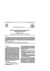
Fig. 3.1.: An example showing how REWARDS works

0x8048118 (line 9). Since 0x8048118 is in the address range of the .rodata section (it is actually the starting address of string “hello world”), ebp-4 can be typed as a pointer, based on the heuristics that instruction executions using similar immediate values within a code or data section are considered type sinks. Note that the type of the pointer is not yet known. At line 10, foo calls 0x8048110. Inside the body of the function invocation (lines 36-38), our algorithm detects a getpid system call (a type sink) with eax being 0x14 at line 36. The return value of the function call is resolved as pid t type (i.e., register eax at line 11 is typed pid t). When eax is copied to address 0x8049124 (a global variable in .bss section as shown in Figure 3.1(c)), the algorithm further resolves 0x8049124 as pid t. Before the function call 0x80480e0 at line 15 (strcpy), the parameters are initialized in lines 12-14. As ebp-4 has been typed as a pointer at line 9, the data flow in lines 12 and 13 dictates that location esp+4 at line 13 is a pointer as well. At line 14, as 0x8049128 is in the global variable section and of a known type, location esp has an unknown pointer type. At line 15, upon the call to strcpy (a type sink),

24 both esp and esp+4 are resolved to char*. Through a backward transitive resolution, 0x8049128 is resolved as char, ebp-4 as char*, and 0x8048118 as char. Also at line 26, inside the function body of strcpy, the instruction “movzbl (%edx),%eax” can be used as another type sink as it moves between the char variables. When the program finishes, we resolve all data types (including function arguments, and those implicit variables such as return address and stack frame pointer) as shown in Figure 3.1(d). The derived types for variables in .rodata, .bss and functions are presented in the figure. Each function is denoted by its entry address. fun 0x080480b4, fun 0x08048110, and fun 0x080480e0 denote foo, my getpid, and strcpy, respectively. The number before each derived type denotes the offset. The variables are listed in increasing order of their addresses. Type stack frame t indicates a frame pointer stored at that location. Type ret addr t means that the location holds a return address. Such semantic information is useful in applications such as vulnerability fuzz. Locations that are not accessed during execution are annotated with the unused type. In fun 0x080480e0, the two char* below the ret addr t represent the two actual arguments of strcpy.

3.2

Detailed Design Now we describe the design of REWARDS. We first identify the type sinks used in

REWARDS and then present the on-line type propagation and resolution algorithm, which will be enhanced by an off-line procedure that recovers more variable types not reported by the on-line algorithm. Finally, we present a method to construct a typed hierarchical view of memory layout.

3.2.1

Type Sinks

A type sink is an execution point of a program where the types (including semantics) of one or more variables can be directly resolved. In REWARDS, we identify three categories of type sinks: (1) system calls, (2) standard library calls, and (3) type-revealing instructions.

25 System calls. Most programs request OS services via system calls. Since system call conventions and semantics are well-defined, the types of arguments of a system call are known from the system call’s specification. By monitoring system call invocations and returns, REWARDS can determine the types of parameters and return value of each system call at runtime. For example, in Linux, based on the system call number in register eax, REWARDS will be able to type the parameter-passing registers (i.e., ebx, ecx, edx, esi, edi, and ebp, if they are used for passing the parameters). From this type sink, REWARDS will further type those variables that are determined to have the same type as the parameter passing registers. Similarly, when a system call returns, REWARDS will type register eax and, from there, those having the same type as eax. In our type propagation and resolution algorithm (Section 3.2.2), a type sink will lead to the recursive type resolution of relevant variables accessed before and after the type sink. Standard library calls. With well-defined API, standard library calls are another category of type sink. For example, the two arguments of strcpy must both be of the char* type. By intercepting library function calls and returns, REWARDS will type the registers and memory variables involved. Standard library calls tend to provide richer type information than system calls. For example, Linux-2.6.15 has 289 system calls, whereas libc.so.6 contains 2,016 functions (note some library calls wrap system calls). Type-revealing instructions. A number of machine instructions that require operands of specific types can serve as type sinks. Examples in x86 are as follows: (1) String instructions perform byte-string operations, such as moving and storing (MOVS/B/D/W, STOS/B/D/W), loading (LOADS/B/D/W), comparison (CMPS/B/D/W), and scanning (SCAS/B/D/W). Note that MOVZBL is also used in string movement. (2) Floating-point instructions operate on floating-point, integer, and binary coded decimal operands (e.g. FADD, FABS, and FST). (3) Pointer-related instructions reveal pointers. For a MOV in­ struction with an indirect memory access operand (e.g., MOV (%edx), %ebx or MOV [mem], %eax), the value held in the source operand must be a pointer. Meanwhile, if the target address is within the range of data sections, such as .stack, .heap, .data, .bss or .rodata, the pointer must be a data pointer. If it is in the range of .text

26 (including library code), the pointer must be a function pointer. Note that the concrete type of such a pointer will be resolved through other constraints.

3.2.2 Online Type Propagation and Resolution Algorithm Given a binary program, our algorithm reveals variable types, including both syntactic types (e.g., int and char) and semantics (e.g., return address), by propagating and resolving the type information along the data flow during program execution. Each type sink encountered leads to both direct and transitive type resolution of variables. More specifically, at the binary level, variables exist in either memory locations or registers without their symbolic names. Hence, the goal of our algorithm is to type these memory addresses and registers. We attach three shadow variables – as the type attribute – to each memory address at the byte granularity (registers are treated similarly): (1) constraint set is a set of other memory addresses that should have the same type as this address; (2) type set stores the set of resolved types of the address1 , including both syntactic and semantic types; (3) timestamp records the birth time of the variable currently in this address. For example, the timestamp of a stack variable is the time when the stack frame is allocated. Timestamps are needed because the same memory address may be reused by multiple variables (e.g., the same stack memory being reused by stack frames of different method invocations). More precisely, a variable instance should be uniquely identified by a tuple . These shadow variables are updated during program execution, depending on the semantics of executed instructions. The on-line type propagation and resolution algorithm, Algorithm 1 on the previous page, takes appropriate actions to resolve types on the fly according to the instruction being executed. For a memory address or a register v, its constraint set is denoted as Sv , which is a set of tuples, and each representing a variable instance that should have the same type as v; its type set Tv represents the resolved types for v; and the birth time of the current variable instance is denoted as tsv . 1

We need a set to store the resolved types because one variable may have multiple compatible types.

27

Algorithm 1 On-line Type Propagation and Resolution 1: /* Sv : constraint set for memory cell (or register) v; Tv : type set of v; tsv : time stamp of v; MOV(v,w): moving v to w; BIN OP(v,w,d): a binary operation that computes d from v and w; Get Sink Type(v,i): retrieving the type of argument/operand v from sink i; ALLOC(v,n): allocating a memory region starting from v with size n – the memory region may be a stack frame or a heap struct; FREE(v,n): freeing a memory region – this may be caused by eliminating a stack frame or de-allocating a heap struct*/ 2: Instrument(i){ 3: case i is a Type Sink: 4: for each operand v 5: T ← Get Sink Type(v, i) 6: Backward Resolve (v, T ) 7: case i has indirect memory access operand o 8: To ← To ∪ {pointer type t} 9: case i is MOV(v, w): 10: if w is a register 11: Sw ← Sv 12: Tw ← Tv 13: else 14: Unify(v, w) 15: case i is BIN OP(v, w, d): 16: if pointer type t ∈ Tv 17: Unify(d, v) 18: Backward Resolve (w, {int, pointer index t}) 19: else 20: Unify3(d, v, w) 21: case i is ALLOC(v, n): 22: for t=0 to n − 1 23: tsv+t ← current timestamp 24: Sv+t ← φ 25: Tv+t ← φ 26: case i is FREE(v, n): 27: for t=0 to n − 1 28: a ← v+t 29: if (Ta ) log (a, tsa , Ta ) 30: log (a, tsa , Sa ) 31: } 32: Backward Resolve(v,T ){ 33: for < w, t > ∈ Sv 34: if (T �⊂ Tw and t ≡ tsw ) Backward Resolve(w,T -Tw ) 35: Tv ← Tv ∪ T 36: } 37: Unify(v,w){ 38: Backward Resolve(v, Tw -Tv ) 39: Backward Resolve(w, Tv -Tw ) 40: Sv ← Sv ∪ {< w, tsw >}; Sw ← Sw ∪ {< v, tsv >} 41: }

28 1. If the current execution point i is a type sink (line 3). The arguments/operands/return values of the sink will be directly typed according to the sink’s definition (Get Sink Type() on line 5)2 . Type resolution is then triggered by calling the recursive method Backward Resolve(). The method recursively types all variables that should have the same type (lines 32-36): It tests if each variable w in the constraint set of v has been resolved as type T of v. If not, it recursively calls itself to type all the variables that should have the same type as w. Note that at line 34, it checks if the current birth timestamp of w is equal to the one stored in the constraint set to ensure the memory has not been re-used by a different variable. If w is re-used (t �= tsw ), the algorithm does not resolve the current w. Instead, the resolution is done by a different off-line procedure (Section 3.2.3). Since variable types are resolved according to constraints derived from data flows in the past, we call this step backward type resolution. 2. If i contains an indirect memory access operand o (line 7), either through registers (e.g., using (%eax) to access the address designated by eax) or memory (e.g., using [mem] to indirectly access the memory pointed to by mem), then the corresponding operand will have a pointer type tag (pointer type t) as a new element in To . 3. If i is a move instruction (line 9), there are two cases to consider. In particular, if the destination operand w is a register, then we just move the properties (i.e., the Sv and Tv ) of the source operand to the destination (i.e., the register); otherwise, we need to unify the types of the source and destination operands because the destination is now a memory location that may have already contained some resolved types. The intuition is that the source operand v should have the same type as the destination operand w if the destination is a memory address. Hence, the algorithm calls method Unify() to unify the types of the two. In Unify() (lines 37-41), the algorithm first unions the two type sets by performing backward resolution at lines 38 and 39. Intuitively, the call at line 38 means that if there are any new types in Tw that are not in Tv (i.e. Tw -Tv ), those new types need to be propagated to v and transitively 2

The sink’s definition also reveals the semantics of some arguments/operands, e.g., a PID.

29 to all variables that share the same type as v, mandated by v’s constraint set. Such unification is not performed if the w is a register to avoid over-aggregation. 4. If i is a binary operation, the algorithm first tests if an operand has been identified as a pointer. If so, it must be a pointer arithmetic operation, the destination must have the same type as the pointer operand and the other operand must be a pointer index – denoted by a semantic type pointer index t (line 18). The semantic type is useful in vulnerability fuzz to overflow buffers. If i is not related to pointers, the three operands shall have the same type. The method Unify3() unifies three variables. It is very similar to Unify() and hence not shown. Note that in cases where the binary operation implicitly casts the type of some operand (e.g., an addition of a float and an integer), the unification induces over-approximation (e.g., associating the float point type with the integer variable). In practice, we consider such cases reasonable and allow multiple types for one variable as long as they are compatible. 5. If i allocates a memory region (line 21), either a stack frame or a heap struct, the algorithm updates the birth time stamps of all the bytes in the region and resets the memory constraint set (Sv ) and type set (Tv ) to empty. By doing so, we prevent the type information of the old variable instance from interfering with that of the new instance at the same address. 6. If i frees a memory region (line 26), the algorithm traverses each byte in the region and prints out the type information. In particular, if the type set is not empty, it is emitted. Otherwise, the constraint set is emitted. Later, the emitted constraints will be used in the off-line procedure (Section 3.2.3) to resolve more variables. Example. Table 3.1 presents an example of executing our algorithm. The first column shows the instruction trace with the numbers denoting timestamps. The other columns show the type sets and the constraint sets after each instruction execution for three sample variables, namely, the global variable g1 and two local variables l1 and l2. For brevity, we abstract the calling sequence of strcpy to a strcpy instruction. After the execution

30 enters method M at timestamp 10, the local variables are allocated and hence both l1 and l2 have the birth time of 10. The global variable g1 has the birth time of 0. After the first mov instruction, the type sets of g1 and l1 are unified. Since neither was typed, the unified type set remains empty. Moreover, l1, together with its birth time 10, is added to the constraint set of g1 and vice versa, denoting they should have the same type. Similar actions are taken after the second mov instruction. Here, the constraint set of l1 has both g1 and l2. The strcpy invocation is a type sink and g1 must be of type char*, the algorithm performs the backward resolution by calling Backward Resolve(). In particular, the variable in Sg1 , i.e. l1, is typed to char*. Note that the timestamp 10 matches tsl1 , indicating the same variable is still alive. Transitively, the variables in Sl1 , i.e. g1 and l2, are resolved to the same type. Note that if the backward resolution was not conducted, we would not be able to resolve the type of l2 because when the move from l1 to l2 (timestamp 12) occurred, l1 was not typed and hence l2 was not typed.

Table 3.1: An example of running the online algorithm. Variable g1 is a global, l1 and l2 are locals. Instruction 10 enter M 11 mov g1, l1 12 mov l1, l2 ... 100 strcpy(g1,)

Tg1 φ φ φ ... {char*}

Sg1 φ {} {} ... {}

tsg1 0 0 0 ... 0

Tl1 φ φ φ ... {char*}

Sl1 φ {} {,} ... {,}

tsl1 10 10 10 ... 10

Tl2 φ φ φ ... {char*}

Sl2 φ φ {} ... {}

tsl2 10 10 10 ... 10

Table 3.2: An example of running the off-line type resolution procedure. The execution before timestamp 12 is the same as Table 3.1. Method N reuses l1 and l2 Instruction ... 12 mov l1, l2 13 Exit M ... 99 Enter N 100 strcpy(g1,..)

Tg1 ... φ φ ... φ {char*}

Sg1 ... {} {} ... {} {}

tsg1 ... 0 0 ... 0 0

Tl1 ... φ φ ... φ φ

Sl1 ... {,} {,} ... φ φ

tsl1 ... 10 10 ... 99 99

Tl2 ... φ φ ... φ φ

Sl2 ... {} {} ... φ φ

tsl2 ... 10 10 ... 99 99

31 3.2.3 Off-line Type Resolution Most variables accessed during the binary’s execution can be resolved by our online algorithm. However, there are still some cases in which, when a memory variable gets freed (and its information gets emitted to the log file), its type is still unresolved. We realize that there may be enough information from later phases of the execution to resolve those variables. We propose an off-line procedure to be performed after the program execution terminates. It is essentially an off-line version of the Backward Resolve() method in Algorithm 1. The difference is that it has to traverse the log file to perform the recursive resolution. Consider the example in Table 3.2. It shares the same execution as the example in Table 3.1 before timestamp 13. At time instance 13, the execution returns from M , deallocating the local variables l1 and l2. According to the online algorithm, their constraint sets are emitted to a log file since neither is typed at that point. Later at timestamp 99, another method N is called. Assume it reuses l1 and l2, namely, N allocates its local variables at the locations of l1 and l2. The birth time of l1 and l2 becomes 99. Their type sets and constraint sets are reset. When the sink is encountered at 100, l1 and l2 are not typed as their current birth timestamp is 99, not 10 as in Sg1 , indicating they are re-used by other variables. Fortunately, the variable represented by < l1, 10 > can be found in the log and hence resolved. Transitively, < l2, 10 > can be resolved as well.

3.2.4 Typed Variable Abstraction Our algorithm is able to annotate memory locations with syntax and semantics. How­ ever, multiple variables may occupy the same memory location at different times and a static variable may have multiple instances at runtime3 . Hence it is important to organize the inferred type information according to abstract, location-independent variables other than specific memory locations. In particular, primitive global variables are represented by 3

A local variable has the same life time of a method invocation, and a method can be invoked multiple times, giving rise to multiple instances.

32 their offsets to the base of the global sections (e.g., .data and .bss sections). Stack variables are abstracted by the offsets from their residence activation record, which is represented by the function name (as shown in Figure 3.1). For heap variables, we use the execution context, i.e., the PC (instruction address) of the allocation point of a heap structure plus the call stack at that point, as the abstraction of the structure. The intuition is that the heap structure instances allocated from the same PC in the same call stack should have the same type. The fields of the structure are represented by the allocation site and field offsets. As an allocated heap region may be an array of a data structure, we use the recursion detection heuristics in [19] to detect the array size. Specifically, the array size is approximated by the maximum number of accesses by the same PC to unique memory locations in the allocated region. The intuition is that array elements are often accessed through a loop in the source code and the same instruction inside the loop body often accesses the same field across all array elements. Finally, if heap structures allocated from different sites have the same field types, we will heuristically cluster these heap structures into one abstraction.

3.2.5 Constructing Hierarchical View of In-Memory Data An important feature of REWARDS is to construct a hierarchical view of a memory snapshot, in which the primitive syntax of individual memory locations, as well as their semantics and the integrated hierarchical structure are visually represented. This is highly desirable in applications like memory forensics as interesting queries (e.g., “find all IP addresses”), can be easily answered by traversing the view. So far, REWARDS is able to reverse engineer the syntax and semantics of data structures, represented by their abstractions. Next, we present how we leverage such information to construct a hierarchical view. Our method works as follows. It first types the top level global variables. In partic­ ular, a root node is created to represent a global section. Individual global variables are represented as children of the root. The edges are annotated with offset, size, primitive

33 type, and semantics of the corresponding children. If a variable is a pointer, the algorithm further recursively constructs the sub-view of the data structure being pointed to, leveraging the derived type of the pointer. For instance, assume a global pointer p is of type T*, our method creates a node representing the region pointed to by p. The region is typed based on the reverse engineered definition of T. The recursive process terminates when none of the fields of a data structure is a pointer. The stack is similarly handled: a root node is created to represent each activation record. Local variables of the record are denoted as children nodes. Recursive construction is performed until all memory locations through pointers are traversed. Note that all live heap structures can be reached (transitively) through a global pointer or a stack pointer. Hence, the above two steps essentially also construct the structural views of live heap data. Our method can also type some of the unreachable memory regions, which represent “dead” data structures (e.g., activation records of previous method invocations whose space has been freed but not reused.) Such dead data is as important as live data as they disclose what had happened in the past. In particular, our method scans the stack beyond the current activation record to identify any pointers to the code section, which often denote return addresses of method invocations. With a return address, the function invocation can be identified and we can follow the aforementioned steps to type the activation record.

3.3

Implementation We implemented REWARDS using PIN-2.6 [69], with 12.1K lines (LOC) of C code

and 1.2K LOC of Python code. REWARDS is able to reveal variable semantics. In our implementation, variable semantics are represented as special semantic tags comple­ mentary to regular type tags such as int and char. Both semantic tags and regular tags are stored in the variable’s type set. Tags are enumerated to save space. The vast diversity of program semantics makes it infeasible to consider them all. Since we are mainly interested in forensics and security applications, we focus on the following semantic tags: (1) file system related (e.g., FILE pointer, file descriptor, file name, file status); (2)

34 network communication related (e.g., socket descriptor, IP address, port, receiving and sending buffer, host info, msghdr); and (3) operating systems related (e.g., PID, TID, UID, system time, system name, and device info). Meanwhile, we introduce some of our own semantic tags, such as ret addr t indi­ cating that a memory location is holding a return address, stack frame t indicating that a memory location is holding a stack frame pointer, format string t indicating that a string is used in format string argument, and malloc arg t indicating an argument of malloc function (similarly, calloc arg t for calloc function, etc.). Note that these tags reflect the properties of variables at those specific locations and hence do not participate in the type information propagation. They can bring important benefits to our targeted applications. REWARDS needs to know the program’s address space mapping, which will be used to locate the addresses of global variables and detect pointer types. In particular, REWARDS checks the target address range when determining if a pointer is a function pointer or a data pointer. Thus, when a binary starts executing with REWARDS, we first extract the coarsegrained address mapping from the /proc/pid/maps file, which defines the ranges of code and data sections including those from libraries, and the ranges of stack and heap (at that time). Then for each detailed address mapping such as .data, .bss and .rodata for all loaded files (including libraries), we extract the mapping using the API provided by PIN when the corresponding image file is loaded.

3.4

Evaluation We have performed two sets of experiments to evaluate REWARDS: one is to evaluate

its correctness, and the other is to evaluate its time and space efficiency. All the experi­ ments were conducted on a machine with two 2.13Ghz Pentium processors and 2GB RAM running Linux kernel 2.6.15. We select 10 widely used utility programs from the following packages: procps-3.2.6 (with 19.1K LOC and containing command ps), iputils-20020927 (with 10.8K LOC and

35 containing command ping), net-tools-1.60 (with 16.8K LOC and containing netstat), and coreutils-5.93 (with 117.5K LOC and containing the remaining test commands such as ls, pwd, and date). The reason for selecting these programs is that they contain many data structures related to the operating system and network communications. We run these utilities without command line option except ping, which is run with a localhost and a packet count 4 option.

3.4.1 Effectiveness To evaluate the reverse engineering accuracy of REWARDS, we compare the derived data structure types with those declared in the program source code. To acquire the or­ acle information, we recompile the programs with debugging information, and then use libdwarf [70] to extract type information from the binaries. The libdwarf library is capable of presenting the stack and global variable mappings after compilation. For in­ stance, global variables scattering in various places in the source code will be organized into a few data sections. The library allows us see the organization. In particular, libdwarf extracts stack variables by presenting the mapping from their offsets in the stack frame and the corresponding types. For global variables, the output by libdwarf is program virtual addresses and their types. Such information allows us to conduct direct and automated comparison. Note that we only verify the types in .data, .bss, and .rodata sections, other global data in sections such as .got, .ctors are not verified. For heap variables, since we use the execution context at allocation sites as the abstract representation, given an allocation context, we can locate it in the disassembled binary, and then correlate it with program source code to identify the heap data structure definition, and finally compare it with REWARDS’s output. Although REWARDS extracts variable types for the entire program address space (including libraries), we only compare the results for user-level code. The result for stack variables is presented in Figure 3.2(a). The figure presents the percentage of (1) functions that are actually executed, (2) data structures that are used in the

36 120 Dynamically Executed Funs Dynamically Exposed Types REWARDS Accuracy 100

Percentage

80

60

40

20

0 e m na st ho

s er us

e am un

e tim up

d

te da

pw

ls

t ta ts ne

ng pi

ps

Benchmark Program

(a) Accuracy on Stack Variables 120 Dynamically Allocated Types Dynamically Exercised Types REWARDS Accuracy

Dynamically Exercised Types REWARDS Accuracy

100

100 80

Percentage

Percentage

80

60

60

40

40

20

20

0

0 s

e

m

e

e

m

na

st

ho

er

us

am

un e

tim

up

t

e

t

ta

te

da

d

pw

ls

ts

ne

s

na

st

ng

pi

ps

ho

er

us

tim

ta

ts

up

ls

ne

ng

pi

ps

Benchmark Program

Benchmark Program

(b) Accuracy on Heap Variables

(c) Accuracy on Global Variables 6e+07

400

REWARDS

REWARDS MemTrace Normal Execution

350

Shadow Memory Consumption (bytes)

5e+07

Execution Time (seconds)

300

250

200

150

100

4e+07

3e+07

2e+07

1e+07 50

0

0

st

ho m

e

na

s

er

us

am

e

e

e

m

(d) Performance Overhead

un

tim

t

ta

te

up

da

d

pw

ls

ts

ne

ng

pi

ps

s

e

na

st

ho

er us

t

e

am

tim

un

up

te

da

d pw

ls ta

ts

ne

ng

pi

ps

Benchmark Program

Benchmark Program

(e) Space Overhead

Fig. 3.2.: Evaluation results for REWARDS accuracy and efficiency

37 executed functions (over all structures declared in those functions), and (3) data structures whose types are accurately recovered by REWARDS (over those in (2)). At runtime, it is often the case that even though a buffer is defined in the source code with size n, only part of the n bytes are used. Consequently, only those used are typed (the others are considered unused). We consider the buffer is correctly typed if its bytes are either correctly typed or unused. From the figure, we can observe that, due to the nature of dynamic analysis, not all functions or data structures in a function are exercised and hence amenable to REWARDS. More importantly, REWARDS achieves an average of 97% accuracy (among these benchmarks) for the data structures that get exercised. For heap variables, the result is presented in Figure 3.2(b), the bars are similarly defined. REWARDS’s output perfectly matches the types in the original definitions when they are exercised. Note some of the benchmarks are missing in Figure 3.2(b) (e.g., date) because their executions do not allocate any user-level heap structures. The result for global variables is presented in Figure 3.2(c), and REWARDS achieves over 85% accuracy. To explain why REWARDS cannot achieve 100% accuracy, we carefully examined the benchmarks and identified the following three reasons: • Hierarchy loss. If a hierarchical structure becomes flat after compilation, we are not able to identify its hierarchy. This happens to structures declared as global variables or stack variables. And the binary never accesses such a variable using the base address plus a local offset. Instead, it directly uses a global offset (starting from the base address of the global data section or a stack frame). In other words, multiple composite structures are flattened into one large structure. In contrast, such flattening does not happen to heap structures. • Path-sensitive memory reuse. This often happens to stack variables. In particular, the compiler might assign different local variables declared in different program paths to the same memory address. As a result, the types of these variables are undesirably unified in our current design. A more thorough design would use a pathsensitive local offset to denote a stack variable.

38 • Type cast. It is possible that a variable type is casted to another one. For example, a float type variable could be casted to an integer type. As such, we will observe different semantic use of one variable, and if this variable is propagated to others, we will over propagate the types. Currently, we do not have a sound solution to this problem, and we just conservatively propagate the types. Despite the imperfect accuracy, REWARDS still suits our targeted application scenar­ ios, i.e., memory forensics and vulnerability fuzzing. For example, although REWARDS outputs a flat layout for all global and stack variables, we can still conduct vulnerability fuzzing because the absolute offsets of these variables are sufficient; and we can still construct hierarchical views of memory images as pointer types can be obtained.

3.4.2

Performance Overhead

We also measured the time and space overhead of REWARDS. We compared it with (1) a standard memory trace tool, MemTrace (shipped along with PIN-2.6) and (2) the normal execution of the program, to evaluate the performance overhead. The result is shown in Figure 4.8. Note the normal execution data is nearly not visible in this figure because they are very small (roughly at the 0.01 second level). We can observe that REWARDS causes slow-down in the order of ten times compared with MemTrace, and in the order of thousands (or tens of thousands) times compared with the normal execution. For space overhead, we are interested in the space consumption by shadow type sets and constraint sets. Hence, we track the peak value of the shadow memory consumption. The result is shown in Figure 3.2(e). We can observe that the shadow memory consumption is around 10 Mbytes for these benchmarks. A special case is ping, which uses much less memory. The reason is that it has fewer function calls and memory allocations, which is also why it runs much faster than the other programs shown in Figure 4.8.

39 3.5

Summary In this chapter, we have presented REWARDS, a reverse engineering system that au­

tomatically reveals data structures in a binary based on dynamic execution. REWARDS involves an algorithm that performs data flow-based type attribute forward propagation and backward resolution. Driven by the type information derived, REWARDS is also capable of reconstructing the structural and semantic view of in-memory data layout. Our evaluation using a number of real-world programs indicates that REWARDS achieves over 80% accuracy in revealing data structures accessed during an execution.

40

4. SIGGRAPH: DISCOVERING DATA STRUCTURE INSTANCES USING GRAPH-BASED SIGNATURES In this chapter, we present the design of SigGraph, the second component in our framework, which aims to discovering data structure instances by scanning memory with the corre­ sponding data structure signatures. To this end, it explores the points-to relation between data structures as signatures and enables the brute force scanning of memory. Brute force scanning requires effective, robust signatures of kernel data structures. Existing approaches often use the value invariants of certain fields as data structure signatures. However, they do not fully exploit the rich points-to relations between data structures. In our technique, a signature is a graph rooted at the subject data structure with edges reflecting the points-to relations with other data structures. We first formally define our problem in Section 4.1, then present the detailed techniques on how we generate such graph based signatures from Section 4.2 to Section 4.5, followed we present the evaluation result in Section 4.7. Finally we conclude in Section 4.8.

Fig. 4.1.: A working example of kernel data structures and a graph-based data structure signature. The triangles indicate recursive definitions

41 4.1

Problem Statement As described in Chapter 2, the goal of SigGraph is to infer the relevant data structure

instances given a memory dump. Basically, it exploits the inter-data structure points-to relations to generate non-isomorphic data structure signatures. To better understand the key idea behind SigGraph, let consider seven simplified Linux kernel data structures, four of which are shown in Figure 4.1(a)-(d). In particular, task struct(TS) contains four pointers to thread info(TI), mm struct(MS), linux binfmt(LB), and TS, respectively. TI has a pointer to TS whereas MS has two pointers: One points to vm area struct(VA) (not shown in the figure) and the other is a function pointer. LB has one pointer to module(MD). At runtime, if a pointer is not null, its target object should have the type of the pointer. Let ST (x) denote a boolean function that decides if the memory region starting at x is an instance of type T and let ∗x denote the value stored at x. Take task struct data structure as an example, we have the following rule, assuming all pointers are not null. STS (x) → STI (∗(x + 0)) ∧ SMS (∗(x + 4)) ∧

(4.1)

SLB (∗(x + 8)) ∧ STS (∗(x + 12))

It means that if STS (x) is true, then the four pointer fields must point to regions with the corresponding types and hence the boolean functions regarding these fields must be true. Similarly, we have the following STI (x) → STS (∗(x + 0))

(4.2)

SMS (x) → SVA (∗(x + 0)) ∧ SFP (∗(x + 4))

(4.3)

SLB (x) → SMD (∗(x + 0))

(4.4)

for thread info, mm struct, and linux binfmt, respectively. Substituting sym­ bols in rule (4.1) using rules (4.2), (4.3) and (4.4), we further have STS (x) → STS (∗(∗(x + 0) + 0)) ∧ SVA (∗(∗(x + 4) + 0))∧ SFP (∗(∗(x + 4) + 4)) ∧ SMD (∗(∗(x + 8) + 0))) ∧STS (∗(x + 12))

(4.5)

42 The rule corresponds to the graph shown in Figure 4.1(e), where the nodes represent pointer fields with their shapes denoting pointer types; the edges represent the points-to relations with their weights indicating the pointers’ offsets; and the triangles represent recursive occurrences of the same pattern. It means that if the memory region starting at x is an instance of task struct, the layout of the region must follow the graph’s definition. Note that the inference of rule (4.5) is from left to right. However, we observe that the graph is so unique that the reverse inference (“bottom-up”) tends to be true. In other words, we can use the graph as the signature of task struct and perform the reverse inference as follows. STS (x) ← STS (∗(∗(x + 0) + 0)) ∧ SVA (∗(∗(x + 4) + 0))∧ SFP (∗(∗(x + 4) + 4)) ∧ SMD (∗(∗(x + 8) + 0)))

(4.6)

∧STS (∗(x + 12))

Different from the global memory mapping techniques (e.g., [25, 30, 52, 53, 55, 56, 58]) SigGraph aims at deriving unique signatures for individual data structures for brute force kernel memory scanning. Hence we face the following new challenges: • Avoiding signature isomorphism Given a static data structure definition, we aim to construct its points-to graph as shown in the task struct example. However, it is possible that two distinct data structures may lead to isomorphic graphs that cannot be used to distinguish instances of the two data structures. Hence our new challenge is to identify the sufficient and necessary conditions to avoid signature isomorphism between data structures. • Generating signatures Meanwhile it is possible that one data structure may have multiple unique signatures, depending on how (especially, how deep) the pointsto edges are traversed when generating a signature. In particular, among the valid signatures of a data structure, finding the minimal signature that has the smallest size while retaining uniqueness (relative to other data structures) is a combinatorial optimization problem. Finally, it is desirable to automatically generate a scanner for each signature that will perform the corresponding data structure instance recognition on a memory image.

43

Fig. 4.2.: SigGraph system overview

• Improving recognition accuracy Although statically a data structure may have a unique signature graph, at runtime, pointers may be null whereas non-pointer fields may have pointer-like values. As a result the data structure instances in a memory image may not fully match the signature. We need to handle such issues to improve recognition accuracy. An overview of the SigGraph is shown in Figure 4.2. It consists of four key compo­ nents: (1) data structure definition extractor, (2) dynamic profiler, (3) signature generator, and (4) scanner generator. To generate signatures, SigGraph first extracts data structure definitions from the OS source code. This is done automatically through a compiler pass (Section 4.2). To handle practical issues such as null pointers and void* pointers, the profiler identifies problematic pointer fields via dynamic analysis (Section 4.5). The signature generator checks if non-isomorphic signatures exist for the data structures and if so, generates such signatures (Section 4.3). The generated signatures are then automati­ cally converted to the corresponding kernel memory scanners (Section 4.4), which are the “product” shipped to users. A user will simply run these scanners to perform brute-force scanning over a kernel memory image (either memory dump or live memory), with the output being the instances of the data structures in the image.

4.2

Data Structure Definition Extraction SigGraph’s data structure definition extractor adopts a compiler-based approach, where

the compiler pass is devised to walk through the source code and extract data structure

44 definitions. It is robust as it is based on a full-fledged language front-end. In particular, our development is in gcc-4.2.4. The compiler pass takes abstract syntax trees (ASTs) as input as they retain substantial symbolic information [71]. The compiler-based approach also allows us to handle data structure in-lining, which occurs when a data structure has a field that is of the type of another structure; After compilation, the fields in the inner structure become fields in the outer structure. Furthermore, we can easily see through type aliases introduced by typedef via ASTs. The output of the compiler pass is the data structure definitions – with offset and type for each field – extracted in a canonical form. The pass is inserted into the compilation work-flow right after data structure layout is finished (in stor-layout.c). During the pass, the AST of each data structure is traversed. If the data structure type is struct or union, its field type, offset, and size information is dumped to a file. To precisely reflect the field layout after in-lining, we flatten the nested definitions and adjust offsets. We note that source code availability is not a fundamental requirement of SigGraph. For a close-source OS (e.g., Windows), if debugging information is provided along with the binary, SigGraph can simply leverage the debugging information to extract the data structure definitions. Otherwise, data structure reverse engineering techniques (e.g., RE­ WARDS [59], TIE [72], or HOWARD [73]) can be leveraged to extract data structure definitions from binaries.

4.3

Signature Generation Suppose a data structure T has n pointer fields with offsets f1 , f2 , ..., fn and types t1 ,

t2 , ..., tn . A predicate St (x) determines if the region starting at address x is an instance of t. The following production rule can be generated for T : ST (x) → St1 (∗(x + f1 )) ∧ St2 (∗(x + f2 )) ∧ ...

(4.7)

∧Stn (∗(x + fn ))

Brute force memory scanning is based on the reverse of the above rule: Given a kernel memory image, we hope to identify instances of a data structure by trying to match the

45 struct A { [0] struct B * a1; ... [12] struct C * a2; ... [18] struct D * a3; }

struct X { ... [8] struct ... [36] struct ... [48] struct ... [54] struct }

c80b20e0: 00 00 00 00 01 20 00 32 c80b20f0: c8 40 30 b0 00 00 00 00 c80b2100: 00 00 c8 41 00 22 00 00

Y

* x1;

BB * x2; CC * x3; DD * x4;

0a 00 00 00 00 ae ff 00 00 10 00 00 c8 40 42 30 00 10 00 00 00 00 00 00

(a) Insufficiency of pointer layout uniqueness

struct B { [0] E * b1; [4] B * b2; }

struct BB { [0] EE * bb1; [4] BB * bb2; }

B/BB

struct D {

...

[4] I * d1;

}

0

B/BB

E/EE struct E { struct EE { ... ...

[12] G * e1; [12] GG * ee1; ... ... [24] H * e3; [24] HH * ee3;

} }

struct DD {

...

[8] II * dd1;

}

+12

G/GG

+4

+24

H/HH

(b) structures of B and BB

(a) definitions

(b) Data structure isomorphism

Fig. 4.3.: Examples illustrating the signature isomorphism problem

right-hand side of the rule (as a signature) with memory content starting at any location. Although it is generally difficult to infer the types of memory at individual locations based on the memory content, it is more feasible to infer if a memory location contains a pointer and hence to identify the layout of pointers with high confidence. This can be done recursively by following the pointers to the destination data structures. As such, the core challenge in signature generation is to find a finite graph induced by points-to relations (including pointers, pointer field offsets, and pointer types) that uniquely identifies a target data structure, which will be the root of the graph. For convenience of discussion, we assume for now that pointers are not null and they each have an explicit type (i.e., not a void pointer). We will address the cases where this assumption does not hold in Section 4.5.

46 As noted earlier, two distinct data structures may have isomorphic structural patterns. For example, if two data structures have the same pointer field layout, we need to further look into the “next-hop” data structures (we call them lower layer data structures) via the points-to edges. Moreover, we observe that even though the pointer field layout of a data structure may be unique (different from any other data structure), an instance of such layout in memory is not necessary an instance of that data structure. Consider Figure 4.3(a), data structures A and X have different layouts for their pointer fields. If the program has only these two data structures, it appears that we can use their one level pointer structures as their signatures. However, this is not true. Consider the memory segment at the bottom of Figure 4.3(a), in which we detect three pointers (the boxed bytes). It appears that SA (0xc80b20f 0) is true because it fits the one-level structure of struct A. But it is possible that the three pointers are instead the instances of fields x2, x3, and x4 in struct X and hence the region is part of an instance of struct X. In other words, a pattern scanner based on struct A will generate false positives on struct X. The reason is that the structure of A coincides with the sub-structure of X. To better model the isomorphism issue, we introduce the concept of immediate pointer pattern (IPP) that describes the one-level pointer structure as a string such that the afore­ mentioned problem can be detected by deciding if an IPP is the substring of another IPP. Definition 4.3.1 Given a data structure T , let its pointer field offsets be f1 , f2 , ..., and fn , pointing to types t1 , t2 , ..., and tn , respectively. Its immediate pointer pattern, denoted as IP P (T ), is defined as follows. IP P (T ) = f1 ·t1 ·(f2 −f1 )·t2 ·(f3 −f2 )·t3 ·...·(fn −fn−1 )·tn . We say an IP P (T ) is a sub-pattern of IP P (R) if g1 · r1 · (f2 − f1 ) · r2 · (f3 − f2 ) · ... · (fn − fn−1 ) · rn is a substring of IP P (R), with g1 >= f1 and r1 , ..., rn being any pointer type. Intuitively, an IP P describes the types of the pointer fields and their intervals. An IP P (T ) is a sub-pattern of IP P (R) if the pattern of pointer field intervals of T is a sub-pattern of R’s, disregarding the types of the pointers. It also means that we cannot distinguish an instance of T from an instance of R in memory if we do not look into the

47 lower layer structures. For instance in Figure 4.3(a), IP P (A) = 0 · B · 12 · C · 6 · D and IP P (X) = 8 · Y · 28 · BB · 12 · CC · 6 · DD. IP P (A) is a sub-pattern of IP P (X). Definition 4.3.2 Replacing a type t in a pointer pattern with “(IP P (t))” is called one t

pointer expansion, denoted as →. − A pointer pattern of a data structure T is a string generated by a sequence of pointer expansions from IP P (T ). For example, assume the definitions of B and D can be found in Figure 4.3(b). IP P (A) = 0 · B · 12 · C · 6 · D B

− → 0 · (0 · E · 4 · B) · 12 · C · 6 · D

(1)

D

− → 0 · (0 · E · 4 · B) · 12 · C · 6 · (4 · I)

(4.8) (2)

Strings (1) and (2) above are both pointer patterns of A. The pointer patterns of a data structure are candidates for its signature. As one data structure may have many pointer patterns, the challenge becomes to algorithmically identify the unique pointer patterns of a given data structure so that instances of the data structure can be identified from memory by looking for satisfactions of the pattern without causing false positives. If efficiency is a concern, the minimal pattern should be identified. Existence of Signature. The first question we need to answer is whether a unique pointer pattern exists for a given data structure. According to the previous discussion, given a data structure T , if its IP P is a sub-pattern of another data structure’s IP P (including the case in which they are identical), we cannot use the one-layer structure as the signature of T . We have to further use the lower-layer data structures to distinguish it from the other data structure. However, it is possible that T is not distinguishable from another data structure R if their structures are isomorphic. Definition 4.3.3 Given two data structures T and R, let the pointer field offsets of T be f1 , f2 , ..., and fn , pointing to types t1 , t2 , ..., and tn , respectively.; the pointer field offsets of R be g1 , g2 , ..., and gm , pointing to types r1 , r2 , ..., and rm , respectively. T and R are isomorphic, denoted as T ⊲⊳ R, if and only if (1) n ≡ m;

48 (2) ∀1 ≤ i ≤ n fi ≡ gi

(2.1)

∧ ( ti ⊲⊳ ri

(2.2)

∨ a cycle is formed when deciding ti ⊲⊳ ri

(2.3)

).

Intuitively, two data structures are isomorphic, if they have the same number of pointer fields (Condition (1)) at the same offsets (2.1) and the types of the corresponding pointer fields are also isomorphic (2.2) or the recursive definition runs into cycles (2.3), e.g., when ti ≡ T ∧ ri ≡ R. Figure 4.3(b) (i) shows the definitions of some data structures in Figure 4.3(a). The data structures whose definitions are missing from the two figures do not have pointer fields. According to Definition 4.3.3, B ⊲⊳ BB because they both have two pointers at the same offsets; and the types of the pointer fields are isomorphic either by the substructures (E ⊲⊳ EE) or by the cycles (B ⊲⊳ BB). Given a data structure, we can now decide if it has a unique signature. As mentioned earlier, we assume that pointers are not null and are not of the void* type. Theorem 4.3.1 Given a data structure T , if there does not exist a data structure R such that IP P (T ) is a sub-pattern of IP P (R), and Assume the sub-pattern in IP P (R) is g1 ·r1 ·(f2 −f1 )·r2 ·(f3 −f2 )·...·(fn −fn−1 )·rn , t1 ⊲⊳ r1 , t2 ⊲⊳ r2 , ... and tn ⊲⊳ rn .

T must have a unique pointer pattern, that is, the pattern cannot be generated from any other individual data structure through expansions. Proof For each data structure R different from T , either condition or is not satisfied according to the preconditions of the theorem. If is not satisfied, IP P (T ) can be used to distinguish T from R. If is not satisfied, there must be an i such that ti is not isomorphic to ri . There must be a minimal k, after k level of expansions, the pointer pattern of ti is different from ri ’s, disregard the type symbols. We say one level of expansion is to expand along all type

49 symbols for one step. IP P (T ) can be considered as the pointer pattern of T with k = 0 level of expansion. Since there are finite number of data structures, we can always identify the maximal among all the k values. Lets denote it as kmax . Hence, the pointer pattern of T after kmax levels of expansions can distinguish T from any other individual data structure. The proof of Theorem 4.3.1 is shown above. Intuitively, the theorem specifies that T must have a unique pointer pattern (i.e., a signature) as long as there is not an R such that IP P (T ) is a sub-pattern of IP P (R) and the corresponding types are isomorphic. If there is an R satisfying conditions and in the theorem, no matter how many layers we inspect, the structure of T remains identical to part of the structure of R, which makes them indistinguishable. In Linux kernels, we have found a few hundred such cases (about 12% of all data structures). Fortunately, most of those are data structures that are rarely used or not widely targeted according to OS security and forensics literature. Note that two isomorphic data structures may have different concrete pointer field types. But given a memory image, it is unlikely for us to know the concrete types of memory cells. Hence, such information cannot be used to distinguish the two data structures. In fact, concrete type information is not part of a pointer pattern. Their presence is only for readability. Consider the data structures in Figure 4.3(a) and Figure 4.3(b). Note all the data structures whose definitions are not shown do not have pointer fields. IP P (A) is a subpattern of IP P (X), B ⊲⊳ BB and C ⊲⊳ CC. But D is not isomorphic to DD because of their different immediate pointer patterns. According to Theorem 4.3.1, there must be a unique signature for A. In this example, pointer pattern (2) in Equation (4.8) is a unique signature. If we find pointers that have such structure in memory, they must indicate an instance of A. Finding the Minimal Signature. Even though we can decide if a data structure T has a unique signature using Theorem 4.3.1, there may be multiple pointer patterns of T that can distinguish T from other data structures. Ideally, we want to find the minimal pattern as it incurs the minimal parsing overhead during brute force scanning. For example, if the offset

50 A

A +18

+18 0

0 +12

B

C

B

C

D +4

B

E

G

D

+4

0

+16

+12

I

+24

H

Fig. 4.4.: If the offset of field e1 (of type struct G) in E is changed to 16, struct A will have two possible signatures (detailed data structure definitions in Figure 4.3)

of field e1 (of type struct G) in E is 16, struct A will have two possible signatures as shown in Figure 4.4. They correspond to the following pointer patterns: 0 · (0 · (16 · G · 8 · H) · 4 · B) · 12 · C · 6 · D

and 0 · B · 12 · C · 6 · (4 · I)

The first one is generated by expanding B and then E, and the second one is generated by expanding D. Either one can serve as a unique signature of A. In general, finding the minimal unique signature is a combinatorial optimization prob­ lem: Given a data structure T , find the minimal pointer pattern of T that cannot be a subpattern of any other data structure R, that is, cannot be generated by pointer expansions from a sub-pattern of IP P (R). The complexity of a general solution is likely in the NP category. In this paper, we propose an approximate algorithm (Algorithm 1) that guarantees to find a unique signature if one exists, though the generated signature may not be the minimal one. It is a breadth-first search algorithm that performs expansions for all pointer symbols at the same layer at one step until the pattern becomes unique. The algorithm first identifies the set of data structures that may have IP P (T ) as their sub-patterns (lines 3-5). Such sub-patterns are stored in set distinct. Next, it performs breadth-first expansions on the pointer pattern of T , stored in s, and the patterns in distinct,

51 Algorithm 2 An approximate algorithm for signature generation Input: Data structure T and set K of all kernel data structures considered Output: The pointer pattern that serves as the signature of T . 1: s= IP P (T ) 2: let IP P (T ) be f1 · t1 · (f2 − f1 ) · t2 · ... · (fn − fn−1 ) · tn 3: for each sub-pattern p=g1 · r1 · (f2 − f1 ) · r2 · (f3 − f2 ) · ... · (fn − fn−1 ) · rn in IP P (R) of each structure R ∈ (K − {T }) with f1