arXiv:cond-mat/0412212v2 [cond-mat.stat-mech] 24 Dec 2004. Reweighting for Nonequilibrium Markov Processes Using. Sequential Importance Sampling ...
Reweighting for Nonequilibrium Markov Processes Using Sequential Importance Sampling Methods
arXiv:cond-mat/0412212v2 [cond-mat.stat-mech] 24 Dec 2004
Hwee Kuan Lee and Yutaka Okabe Department of Physics, Tokyo Metropolitan University, Hachioji, Tokyo 192-0397, Japan (Dated: February 2, 2008) We present a generic reweighting method for nonequilibrium Markov processes. With nonequilibrium Monte Carlo simulations at a single temperature, one calculates the time evolution of physical quantities at different temperatures, which greatly saves the computational time. Using the dynamical finite-size scaling analysis for the nonequilibrium relaxation, one can study the dynamical properties of phase transitions together with the equilibrium ones. We demonstrate the procedure for the Ising model with the Metropolis algorithm, but the present formalism is general and can be applied to a variety of systems as well as with different Monte Carlo update schemes. PACS numbers: 64.60.Ht, 75.40.Gb, 05.10.Ln
The Monte Carlo simulation has served as a standard method to treat many body problems in statistical physics [1]. Metropolis et al. [2] used the importance sampling, which generates the states with a probability proportional to the Boltzmann factor. The importance sampling method can be considered as a reweighting technique in a sense that one samples a trial distribution and takes an average for the true distribution with reweighting. A more direct way of reweighting is found in the histogram reweighting method due to Ferrenberg and Swendsen [3], where equilibrium thermal averages for a range of temperatures can be calculated from a single simulation. This method greatly improved the efficiencies of Monte Carlo simulations, however, the histogram reweighting technique has to be used only to calculate equilibrium properties. Recently, nonequilibrium relaxation method has been successfully applied to the study of critical phenomena [4, 5, 6, 7]. In the nonequilibrium relaxation method, simulations were performed for several temperatures; the critical temperature, the dynamical exponent and other quantities are estimated using the scaling behavior of nonequilibrium process. If we combine the strength of nonequilibrium relaxation method with a reweighting technique, we can expect an effective method of simulation. In this paper, we will present a generic reweighting method that is applicable to both equilibrium and nonequilibrium systems. With reweighting at nonequilibrium, only a simulation at a single temperature is required. Our method of reweighting may also be applicable in a multitude of other nonequilibrium processes, such as the contact process [8] and the driven diffusive systems [9]. Reweighting at nonequilibrium can be easily understood as follows. Consider every simulation up to the tth Monte Carlo step as a sequence of states (or path), ~xt = (σ1 , σ2 , · · · , σt )
(1)
where σt is the system configuration at time t. Hereafter, we refer to Monte Carlo step simply as the time of simulation. Such path ~xt can be generated using any Monte
Carlo method at a temperature T . The objective is to calculate the relative probability of generating the same path ~xt at another temperature T ′ . Suppose many simulations were performed at an inverse temperature β = 1/kB T to obtain a set of paths ~xjt , j = 1, · · · , n. (From now on, β will be sometimes referred to as temperature). Dynamical thermal average of some quantity Q(t) can be obtained by hQ(t)iβ = Pn (1/n) j=1 Q(~xjt ). To calculate the dynamical thermal average at another temperature β ′ , the measured quantity Q(~xjt ) has to be reweighted with a set of weights wtj . For the same set of paths ~xjt , the thermal average at β ′ is obtained as hQ(t)i
β′
=
n X j=1
wtj Q(~xjt )/
n X
wtj
(2)
j=1
Although not labeled explicitly in Eq. (2), the set of weights wtj depend on the simulation temperature β and the new temperature β ′ . To calculate the weights, the following algorithm is implemented for each path ~xjt , j = 1, · · · , n. 1. Assume that the Monte Carlo simulation is carried out at a temperature β, and a path ~xjt = (σ1j , · · · , σtj ) for some arbitrary time t is obtained. 2. To go from time t, let σ ′j be a trial configuration j and T (σ ′ |σtj ) be the probability to select this configuration. If the trial move is accepted with the j acceptance probability Aβ (σ ′ |σtj ), then the new j configuration at t + 1 becomes σt+1 = σ ′j . If the j move is not accepted, σt+1 = σtj . 3. In terms of the transition probability j j |σtj ) = |σtj ), we may write as Pβ (σt+1 Pβ (σt+1 j j T (σ ′ |σtj )Aβ (σ ′ |σtj ) if the move is accepted and, j j j Pβ (σt+1 |σtj ) = T (σ ′ |σtj )[1 − Aβ (σ ′ |σtj )] otherwise. j can be obtained 4. Then the appropriate weights wt+1
2 by j wt+1 =
j |σtj ) Pβ ′ (σt+1 j Pβ (σt+1 |σtj )
wtj with w1j = 1
(3)
5. Repeat steps 2 to 4 until t reaches some predetermined maximum simulation time. For each path ~xjt , j = 1, · · · , n, these steps are repeated. Step 2 is simply the standard Monte Carlo procedure of acceptance and rejection. Step 3 calculates the transition probability after the decision on acceptance was made. Step 4 updates the appropriate weight. In this method, essentially the usual Monte Carlo update is carried out, and at the same time the weights were updated. The proof of Eq. (3) involves two ingredients, the Sequential Importance Sampling (SIS) [10, 11, 12] method and a generic Monte Carlo method. A brief description of SIS method will be discussed here. The SIS method assumes that the distribution for a multi-dimensional state ~xt = (σ1 , σ2 , · · · , σt ) is known and let it be denoted by πt (~xt ). Implementation of the SIS algorithm is as follows: j j 1. Draw σt+1 from a trial distribution gt+1 (σt+1 |~xt ) j ). to form ~xjt+1 = (~xjt , σt+1
2. The importance weight at t + 1 is given by j wt+1 =
πt+1 (~xjt+1 ) wtj j j j πt (~xt )gt+1 (σt+1 |~xt )
(4)
The key to understanding the reweighting method is to realize that in a Monte Carlo simulation, the time sequence ~xjt is sampled from the true probability distribution of the path at some temperature β. The Monte Carlo method is Markovian and the probability of obtaining the path is given by
which is as presented in Eq. (3). The initial condition in Eq. (3) is w1j = 1 because the initial system configuration is chosen from a distribution independent of temperature. To illustrate how the reweighting algorithm is implemented, we use the ferromagnetic Ising model on a square lattice. Its Hamiltonian is given by X sk sl (10) H=− hkli
where the sum is over nearest neighbors and sk takes the values ±1. Periodic boundary conditions are used on a L × L lattice. We use the single spin flip update with the Metropolis acceptance rate, but other update schemes are also applicable. The simulation is performed at β; the objective is to reweight it to β ′ . The system configuration σ is denoted by the states of all spins, σ = {s1 , · · · , sN }, where N is the total number of sites. The initial system configuration at time t = 1 is set to sk = +1 for all k = 1, · · · , N . Hence w1j = 1 for j = 1, · · · , n; recall that j is used for indexing different paths. For each path ~xjt = (σ1j , σ2j , · · · , σtj ), 1. Choose a spin and flip it with probability, j Aβ (σ ′ |σtj ) = min[1, exp(−β∆E)]. Here, ∆E is the energy change due to the spin flip. 2. At this point, there are three possible outcomes, (a) If ∆E ≤ 0, the proposed spin flip is always j accepted; and we obtain wt+1 = wtj × 1. (b) If ∆E > 0 and the proposed spin flip is acj cepted, we obtain wt+1 = wtj × exp(−(β ′ − β)∆E).
(5)
(c) If ∆E > 0 and the proposed spin flip j is rejected, we obtain wt+1 = wtj × ′ (1 − exp(−β ∆E))/(1 − exp(−β∆E)).
j where Pβ (σtj |σt−1 ) is the probability of getting a system configuration σtj at time t given that the system configuj ration is σt−1 at an earlier time t − 1. P (σ1j ) is the probability of choosing the initial configuration. One may obtain the probability distribution function, Pβ ′ (~xjt ), of the path at another temperature β ′ using Pβ (~xjt ) as a trial distribution. The SIS method can then be used by defining the following quantities in Eq. (4) as
3. Although the weights should be updated for every single spin flip move, thermal quantities may be recorded only once per N single spin flip steps, for example, to save memory. Let τ be the time in unit of Monte Carlo steps per site (MCSS); weights wτj j and moments of magnetization (mλ )τ , λ = 1, 2, 4 (i.e. m, m2 and m4 moments) are accumulated into P P P j j the sums, j wτj , j (mλ )τ and j (mλ )τ wτj .
j ) · · · Pβ (σ2j |σ1j )P (σ1j ) Pβ (~xjt ) = Pβ (σtj |σt−1
πt+1 (~xjt+1 ) ≡ Pβ ′ (~xjt+1 )
(6)
πt (~xjt ) ≡ Pβ ′ (~xjt ) j gt+1 (σt+1 |~xjt )
≡
(7)
j Pβ (σt+1 |~xjt )
(8)
The requirement for the Monte Carlo process being j j Markovian implies Pβ (σt+1 |~xjt ) = Pβ (σt+1 |σtj ), and using Eq. (5), we obtain j wt+1 =
Pβ ′ (~xjt+1 ) j |~xjt ) Pβ ′ (~xjt )Pβ (σt+1
wtj =
j Pβ ′ (σt+1 |σtj ) j Pβ (σt+1 |σtj )
wtj
(9)
We carried out many simulations to obtain a set of paths ~xjt , j = 1, · · · , n. Finally, the dynamical thermal averages for each time τ , hm(τ )λ iβ ′ , for example, can be calculated from the accumulated sums using Eq. (2). In practice reweighting to many temperatures β1′ , β2′ , · · · were made at the same time in a single run. Fig. 1 shows plots of the temporal evolution of magnetization for several reweighted temperatures from simulations at a single temperature T = 2.270 (bold line) on the L = 64 square lattice. These data were generated with three independent runs to estimate error bars; for each
3
< m(τ) > / < m(τ) >
2
0.7
2 0.55
0.4 0.3 0.45
0.2 1500
0
100
1.05
-4
-5×10
-3
2000
-1×10 0
1000
τ (MCSS)
10000
FIG. 1: Plot of magnetization for reweighted temperatures from simulations at a single temperature T = 2.270 (bold line). From top to bottom, T =2.268, 2.269, 2.270, 2.271, 2.272. System size is L = 64. τ represents Monte Carlo time in units of MCSS. Insert shows the region between 1000 to 2000 MCSS with representative error bars.
run, averages were taken over 2.94 × 10⁵ samples. Effective reweighting temperature range is about ∆T = 0.002 for L = 64. Insert shows the region between 1000 and 2000 MCSS with representative error bars. Error bars become larger as reweighting is done at temperatures further away from the simulation temperature. Similar to the argument put forward by Ferrenberg and Swendsen [3], reweighting is effective when the distributions Pβ (~xjt ) and Pβ ′ (~xjt ) have sufficient overlaps. An additional simulation, performed at T = 2.268, for example, yields the results consistent with the reweighted ones within statistical errors. A more detailed comparison of actual and reweighted data will be discussed shortly. The ratio of the moments of the order parameter is used for the analysis of the phase transition [13]. Fig. 2 shows plots of hm(τ )4 i/hm(τ )2 i2 for several reweighted temperatures from simulations at T = 2.270. From top to bottom, T = 2.272, 2.271, 2.270, 2.269, 2, 268, 2.267. The lattice size was L = 32 and accuracy of reweighting was checked by performing an additional simulation at T = 2.268. This simulation was then reweighted to T = 2.270 and compared to the curve from the original simulation. The dashed line in Fig. 2 shows hm(τ )4 i/hm(τ )2 i2 at T = 2.270 reweighted from T = 2.268. Insert shows that the difference between the dashed line and solid line is about 5 × 10⁻⁴ while error bars of hm(τ )4 i/hm(τ )2 i2 are of the order 10−3 . Averages were taken with 1.28 × 10⁶ samples. The systematic errors due to reweighting are smaller than the statistical errors for this temperature shift. Equilibrium properties can be calculated using reweighting by performing the simulation up to equilibrium and beyond, and then disregard data at nonequilibrium. In this domain, our reweighting method yields the same results as the histogram reweighting [3] method. Fig. 3 shows Binder’s cumulants [13] for L = 32, L = 48,
10
200
400
600
100
800
1000
τ (MCSS)
FIG. 2: Values of hm(τ )4 i/hm(τ )2 i2 for reweighted temperatures from simulations at T = 2.270. From top to bottom, T = 2.272, 2.271, 2.270, 2.269, 2, 268, 2.267. To check the range of reweighting, an additional simulation was performed at T = 2.268 and reweighted to T = 2.270. Dashed line shows hm(τ )4 i/hm(τ )2 i2 at T = 2.270 reweighted from T = 2.268. Insert shows that the difference between the dashed line and solid line is about 5 × 10⁻⁴ while error bars on hm(τ )4 i/hm(τ )2 i2 are of the order 10−3 . The system size is L = 32. τ represents Monte Carlo time in units of MCSS. 0.614
2 2
1000
10
5×10
4
0.50
-4
1.10
0.612
0.610
4
0.5
1.15
1 - / 3
m(τ)
0.6
L = 32 L = 48 L = 64 L = 80
0.608
0.606 2.268
2.269
2.270
2.271
2.272
T FIG. 3: Binder’s cumulants for L = 32, L = 48, L = 64 and L = 80. Simulation temperatures are indicated by arrows, T = 2.27 for L = 32, 48, T = 2.269 for L = 64, 80. Error bars when not shown are smaller than the size of the symbols.
L = 64 and L = 80. Simulations were performed at one temperature for each lattice size. The crossing of curves with different sizes yields the determination of the critical temperature Tc . In the present case, we confirm that the exact Tc = 2.2691 · · · is well reproduced. Simulation temperatures are indicated by arrows; T = 2.27 for L = 32, 48 and T = 2.269 for L = 64, 80. The reweighting temperature range we used is ∆T = 0.004 for L = 32, 48, ∆T = 0.002 for L = 64 and ∆T = 5 × 10⁻⁴ for L = 80. Error bars were generated with several independent simulations, and they are smaller than the size of the symbols. This suggests that the effective reweighting temperature
4 1.20
1.15
1.10
4
2
< m(τ) > / < m(τ) >
2
at z = 2.143 ± 0.063 for L = 64 and 80. We have given the error bars on z from the variance of the estimate of z by a set of independent runs. Simulations were performed at relatively small system sizes compared to more extensive simulations [17, 18]. Considering the effect of corrections to scaling, our value of z is, within error bars, approaching the values that were previously reported z = 2.16 ∼ 2.17 [17, 18, 19].
1.05
0.001
0.01
-z
τL
0.1
1
FIG. 4: Finite-size scaling plot of hm(τ )4 i/hm(τ )2 i2 for L = 32, 48, 64 and 80 at Tc = 2.2691 · · ·. The dynamical exponent is chosen as z = 2.143 for this plot.
range is actually larger than the temperature range we used in our calculations. For each independent run, averages were taken with 1.28 × 10⁶ samples for L = 32, 2.59 × 10⁵ samples for L = 48, 1.28 × 10⁵ samples for L = 64 and 4 × 10⁴ samples for L = 80. The dynamical finite-size scaling [14] can be used in combination with nonequilibrium relaxation [15, 16]. Making use of the scaling form [17], hm(τ )4 i/hm(τ )2 i2 = g(τ L−z )
(11)
the dynamical exponent z can be estimated by plotting hm(τ )4 i/hm(τ )2 i2 versus τ L−z at the known Tc = 2.2691 · · · value (Fig. 4). The estimate of z is obtained when curves of different sizes are collapsed into a single curve. The best fit for data collapse is obtained by choosing z = 2.143 ± 0.063 for all the data shown in Fig. 4. For the curves of L = 32 and 48, the best fit occurs at z = 2.11 ± 0.02. The best fit is obtained at z = 2.138 ± 0.039 for L = 48 and 64, and
[1] D. P. Landau and K. Binder, A Guide to Monte Carlo Simulations in Statistical Physics, (Cambridge University Press, Cambridge, 2002). [2] N. Metropolis, A. W. Rosenbluth, M. N Rosenbluth, A. M. Teller and E. Teller, J. Chem. Phys. 21, 1087 (1953). [3] A. M. Ferrenberg and R. H. Swendsen, Phys. Rev. Lett. 61, 2635 (1988). [4] H. J. Luo, L. Schulke and B. Zheng, Phys. Rev. Lett. 81, 180 (1998). [5] B. Zheng, M. Schulz and S. Trimper, Phys. Rev. E 59, R1351 (1999). [6] N. Ito, K. Hukushima, K. Ogawa and Y. Ozeki, J. Phys. Soc. Jpn. 69, 1931 (2000). [7] Y. Ozeki, K. Ogawa and N. Ito, Phys. Rev. E 67, 026702 (2003). [8] M. Henkel and H. Hinrichsen, J. Phys. A 37, R117
To summarize, we have presented a reweighting method for nonequilibrium Markov processes. We have shown the basis of this method starting from the formulation of the SIS method. As a demonstration, we have used the Ising model on a square lattice. With the nonequilibrium simulation at a single temperature, we can determine the critical temperature and critical exponents using finite-size scaling. The nonequilibrium simulation for large enough systems [6, 7] is one way to extract dynamical and also static properties without worrying about finite-size effects. The systematic analysis of finitesize effects, the finite-size scaling [14, 15, 16], is another way of studying nonequilibrium relaxation. The nonequilibrium reweighting is useful when it is combined with the latter approach. We should note that this method is neither restricted to single spin flip updates nor the Ising model. This method is applicable, in principle, whenj j |σtj )/Pβ (σt+1 |σtj ) ever the ratio of probabilities Pβ ′ (σt+1 can be calculated numerically. It should be applicable with other Monte Carlo update schemes such as the cluster update schemes [20, 21] as well as the N -fold way method [22]. We should mention that Dickman [23] proposed a similar reweighting method for the application to the contact process. However, our formalism is more extensive and general. This work was supported by a Grant-in-Aid for Scientific Research from the Japan Society for the Promotion of Science. The computation of this work has been done using computer facilities of the Supercomputer Center, Institute of Solid State Physics, University of Tokyo.
(2004), [9] B. Schmittmann and R. K. P. Zia, in Phase Transitions and Critical Phenomena, edited by C. Domb and J. L. Lebowitz (Academic Press, New York, 1995) Vol. 17, p. 1. [10] J. S. Liu and R. Chen, J. Amer. Stat. Assoc. 93, 1032 (1998). [11] J. L. Zhang and J. S. Liu, J. Chem. Phys. 117, 3492 (2002); A brief introduction of the SIS method is given in Appendix. [12] A. Doucet, N. De Freitas and N. Gordon, Sequential Monte Carlo Methods in Practice, (Springer, New York, 2001). [13] K. Binder, Z. Phys. B 43, 119 (1981). [14] M. Suzuki, Prog. Theor. Phys. 58, 1142 (1977). [15] M. Kikuchi and Y. Okabe, J. Phys. Soc. Jpn. 55, 1359
5 (1986). [16] Y. Y. Goldschmidt, Nucl. Phys. B 285, 519 (1987). [17] Y. Okabe, Y. Tomita and K. Kaneda, J. Phys. Soc. Jpn. 69, Suppl. A, 199 (2000). [18] N. Ito, Physica A 196, 591 (1993). [19] M. P. Nightingale and H. W. J. Bl¨ ote, Phys. Rev. Lett. 76, 4548 (1996).
[20] R. H. Swendsen and J. S. Wang, Phys. Rev. Lett. 58, 86 (1987). [21] U. Wolff, Phys. Rev. Lett. 62, 361 (1989). [22] A. B. Bortz, M. H. Kalos and J. L. Lebowitz, J. Comput. Phys. 17, 10 (1975). [23] R. Dickman, Phys. Rev. E 60, R2441 (1999).