Road Crash Proneness Prediction using Data Mining Richi Nayak
Daniel Emerson
Justin Weligamage
Queensland University of Queensland University of Department of Transport and Technology, Brisbane, Technology, Brisbane, Main Roads Queensland Queensland, Australia,4000 Queensland, Australia, 4000 477 Boundry St +61731381976 +61731381976 Spring Hill, QLD, 4000 +61738343843
[email protected] d.emerson@connect.
qut.edu.au
ABSTRACT Developing safe and sustainable road systems is a common goal in all countries. Applications to assist with road asset management and crash minimization are sought universally. This paper presents a data mining methodology using decision trees for modeling the crash proneness of road segments using available road and crash attributes. The models quantify the concept of crash proneness and demonstrate that road segments with only a few crashes have more in common with non-crash roads than roads with higher crash counts. This paper also examines ways of dealing with highly unbalanced data sets encountered in the study.
Categories and Subject Descriptors J.2 [Computer Applications]: Physical Sciences and Engineering - data mining, experimentation, performance, reliability
General Terms Algorithms, Design, Reliability, Experimentation, Verification
Keywords Road Crashes, Data Mining, Crash proneness, Predictive data mining
1. INTRODUCTION The efficiency of road transport has an impact on both the environmental sustainability and the economic competence of our societies. Traffic delays and crashes incur costs that have environmental and economic impacts, and often tragic human outcomes. Road design standards aim to specify safe roads. A particular road design is derived by selecting appropriate road attributes for the prevailing conditions. Decisions are made to manage known crash-prone road segments: firstly performing temporary measures such as speed reduction and signage; and subsequently by works including seal replacement, barriers, geometric changes and so on. Being able to differentiate between crash prone and non-crash prone road segments in these situations would be of use to road asset managers in their decision making process. Permission to make digital or hard copies of all or part of this work for personal or classroom use is granted without fee provided that copies are not made or distributed for profit or commercial advantage and that copies bear this notice and the full citation on the first page. To copy otherwise, to republish, to post on servers or to redistribute to lists, requires prior specific permission and/or a fee. EDBT 2011, March 22--24, 2011, Uppsala, Sweden. Copyright 2011 ACM 978-1-4503-0528-0/11/0003\ ...\$10.00}
Noppadol Piyatrapoomi Department of Transport and Main Roads Queensland 477 Boundry St Spring Hill, QLD 4000 +61738343843
justin.z.weligamage@ Noppadol.A.Piyatrapoo tmr.qld.gov.au
[email protected] This paper presents a road-crash case study primarily deploying decision trees to augment that decision making process. The resulting road segment classification, using road segment crash count as a measure, identifies crash count ranges that define a road section as crash prone. The foundation study was performed by Shankar et al, using statistical methods [1]. While the DM models were based on crash and road data from the Queensland Department of Transport and Main Roads (QDTMR), the methodology can be applied by other road authorities by developing models with their own data. The preliminary stage of our study [2] demonstrated that data mining algorithms, based on the road attributes, can differentiate between road segments with crashes and those without crashes. The subject of this paper is the second and third stages of modeling, which demonstrate that the best division is not a crash vs. no-crash model, but a higher threshold of no-crash and low crash counts vs. higher crash counts. Analysis of models quantifies the crash prone threshold. For this dataset, model efficiencies indicate that best road segment crash-proneness threshold was four to eight crashes in a four year period (that is, one to two crashes per annum). Results indicate that road segments with low crash counts have more in common with roads without crashes than they have with roads that have high crash rates. This understanding allows road asset managers to focus their efforts on crash-prone roads, leaving other sections of the agency to focus on mitigating the non-road causes of crashes. Difficulties were encountered in the interpretation of statistics in assessment of models. Some of the model datasets in the testing range had unbalanced logistic classes, where one class was excessively larger in instance count than other class. Conflict between results demonstrated that some of the model assessment statistics were ineffective in this situation. This paper discusses some of the model assessment strategies used to assess the models built on these unbalanced datasets. The paper structure is as follows. Section 2 examines road attributes and related work. Section 3 traces data development and proposes the data mining methodology for predicting crash proneness. Section 4 examines the results. Section 5 provides a summary of the outcome of the models and proposes future directions.
2. BACKGROUND AND RELATED WORK Data mining methods are increasingly being used in road crash studies [3, 4]. Studies relevant to our paper include: Shankar,
Milton & Mannering [1] which provides the foundation work based on statistical methods; Chang and Chen [5] which establishes decision trees for study of traffic accidents and road variables; Wong & Chung [6] which demonstrates data mining models using crash counts; and Anderson [7] which utilizes clustering to identify accident hotspots. Our study uses tree model efficiencies as an indicator of the best dataset partitioning between crash prone and non-crash prone roads. To our best knowledge, no studies have used the characteristics of data mining to explore the value of the crash count indicator for defining the non-crash prone zone between the boundaries of roads without crashes, and roads that are crash prone.
extend our model of road segment having-crashes, a method of measuring the magnitude of crash proneness of road segments was required, and in the data preparation stage, road segment crash counts were calculated and provided the required measure.
The goal of road design is to apply known engineering principles for traffic flow density and speed for minimal crash probability within the contexts of safety, cost, driver expectation, and economic and environmental parameters [8]. The attributes, involved in the design process and available for the study, can be grouped in the following major areas: structural strength and flexibility (deflection), functional design, surface properties, surface distress, surface wear, traffic, roadway features and geometry, and crash parameters.
Two sets of the crash-proneness datasets were created: the moreinclusive crash/no crash dataset and the smaller crash only data subset. Phase 1 modeling used the crash proneness datasets developed from the crash/no crash dataset. The preliminary goal of this model was to distinguish between road segments with crashes from road segments without crashes and required noncrash instances. Inspired by the zero-altered counting process from Shankar et al. [1], the zero-altered counting set, an imaginary set of non-crash instances with road characteristics from the non-crash roads, was created to provide comparative attributes for the crash-no/crash differentiation.
This study selects attributes from functional design, surface properties, surface distress, surface wear and roadway features.
3. THE PROPOSED CRASH PRONENESS METHOD To conform to industry-standard processes, the CRISP-DM (CRoss-Industry Standard Process for Data Mining) framework [9] was used to guide the study through development of its data exploration, data preparation, model deployment and model assessment and evaluation. The DM goal was to improve our prior model [2] that predicted the crash status of road segment from road attributes. The improvement strategy was to prepare and assess a series of new crash-proneness datasets by moving the binary crash threshold higher into the crash count range (e.g. 0-2 crashes vs. more than 2 crashes and so on). Assessment was accomplished through predictive model accuracy measures and examination of classes of cluster model and the crash count ranges within the classes. .Understanding business problems, data and pre-processing In the CRISP_DM stage of understanding business problems, the study was engaged in the discovery activities guided by the goal of seeking to contribute to knowledge that would make roads safer, specifically in the management of road surface friction. The specific DM goal was to produce a more accurate model than that of our prior stage of modeling [1]. This model had contributed substantially to the understanding data phase, by demonstrating that the road crash data could produce predictive road crash models able to distinguish between road segments with and without crashes based on road & traffic attributes. Attributes such as skid resistance and texture depth were found to have strong relationship with roads having crashes, and wet & dry roads were found to have differing distributions of crash with respect to skid resistance and traffic rates. We challenged the assumption of the linear relationship between road segment crash count and traffic rates. The inspiration for this paper came from the work of Shankar, Milton & Mannering [10] who stated that some roads, due to design or condition, have higher crash rates than others, and the term crash proneness was adopted. Since the objective was to
The new road segment crash count attribute was benchmarked against other attributes found to correlate with prior findings, and was used to generate six new crash-proneness datasets, each with a progressively higher crash count division for non-crash prone and crash prone classes. The strategy was to select the threshold from the model assessed with the highest classification rate near the crash/no crash boundary as the best threshold for making the crash-proneness division.
Phase 2 modeled with the crash only data subset. Datasets from the road authority contained the full 42,388 crash instances from the four year period 2004-2007. Crash selections were limited by the requirement to model the sparse skid resistance (F60) attribute, providing a final crash set of 16,750 crashes and their road attributes. The finalized dataset provided 16,750 crash-road instances and 16,155 no-crash instances. The series of crash-proneness datasets was developed with the target variable for each set derived from a progressively higher crash count threshold. Crash prone 2, for example, compares 1km road segment attributes from roads, with 0,1 or 2 crashes (4 year) as the non-crash prone road segments, roads with 3 crashes and above as the crash prone road segments. Using this method, a series of binary crash threshold variables derived from the crash counts was developed for each of the thresholds of 2,4,8,12,16,32 and 64 road segment crashes respectively. Table 1 details the six crash-only datasets. The crash prone instance counts are reflective of the diminishing instance count as the crash count threshold increases. Table 1. Crash prone threshold target values of modeling phase 2
Target label
Road segment crash count threshold
CP-2
>2
3548
13202
16750
CP-4
>4
5904
10846
16750
CP-8
>8
8677
8073
16750
CP-16
>16
12348
4402
16750
CP-32
>32
15471
1279
16750
CP-64
>64
16576
174
16750
Non-crash prone instances
Crash prone instances
Total instance count
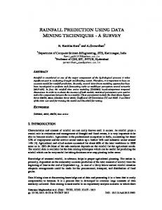
The distribution of crashes in Figure 1 shows that most roads with crashes have very low crashes counts, and the number drops exponentially as the crash count increases, thus exacerbating the imbalance between the classes in the higher thresholds. The chart also shows that the distribution is fairly constant from year to year.
Phase 1 and 2 deployed the following tree algorithms;
Scatterplot of 2004, 2005, 2006, 2007 vs Year Crash Count 1400
Variable 2004 2005 2006 2007
Crash Instance Count
1200 1000 800 600 400 200 0 0
5
10
15 20 Year Crash Count
25
30
and comparing the results. The third stage deployed clustering on the crash-only dataset for the optimal crash-prone threshold derived from phases 1 and 2. The aim was to compare the crashcount ranges within each clustered instance set, in the search of low, mid or high crash count distributions to support the noncrash prone & crash prone concept.
35
Figure 1. Distribution of annual crash counts The study was motivated to transition from the crash/no crash models and focus on the crash only subset models for two reasons. The first reason was to remove the zero crash component of the dataset because the limited distribution of traffic density in non-crash road segments. The AATD distribution violates the basic modeling assumption of independent identically distributed observations [10] and has the potential to adversely affect models. The second reason is that modeling with crash only dataset allowed utilization of the richer attribute set that belongs to the road attributes of crashonly data for later work. Thus phase 2 jettisoned the no-crash instances and focused on crash proneness models derived from the crash only dataset. The dataset used in these models included a total of 16,750 crash-road instances. Data preprocessing was a continual process throughout the study. All variables underwent the standard pre-processing and distribution testing by examining the relevance of missing values and relevance of distribution skew. Transformations involving information loss, such as discretization, were avoided and interval values were retained. Most transformations performed poorly, and thus original values were used, and since trees, which are not sensitive to missing values, were the predominant algorithm, the missing values were treated as valid data. Most road attributes contributed, some in a small way, and were included in the models.
3.1 Model design and configuration The aim of modeling was to determine if roads in the low crash count region had characteristics more in common with non-crash roads than crash roads. Thus a series of crash prone data sets with their progressively increasing crash prone/non crash prone threshold were tested and assessments compared. Our expectation was that crash prone models with a threshold of a few crashes would show better classification rates than the traditional crash/no crash models, because low-crash roads would have similar road attributes to non-crash roads. Modeling was conducted over three phases: firstly deploying and assessing predictive models on the crash/no crash datasets; then repeating the procedures with the crash-only data subset;
decision trees, using with chi-square test on a Boolean target, with the objective of obtaining the minimum class classification rates as the model assessment. regression trees, using the f-test on a target configured as interval, to obtain the coefficient of determination (rsquared) for use in the assessment of predictive accuracy of the model. Interval models tended to be more accurate but with less compact models.
During the configuration process, a series of modeling tests was conducted on the data to determine a suitable tree size that did not significantly truncate the tree. This phase of the study was in the discovery stage; therefore highly accurate outcomes were not sought. Thus the training/validation method was used because correlations between the training and validation plots provided by this method are good indicators of the raw model quality, an aspect that is obscured by the use of high performance methods such as cross-validation, boosting, bagging and so on. Several supporting models, including logistic regression, neural networks, and naïve Bayesian models, were configured with 10 times cross-validation. Models derived from decision trees were shown to be the most comprehensible and compact while still providing acceptable performance. Phase 3, deploying clustering using the optimal model of eight crashes per road segment (4 year data period), used simple kmeans as the method, configured to provide 32 clusters.
3.2 Model Evaluation Assessing the built predictive tree models in Phases 1 and 2 presented a problem because of the extreme imbalance between the class instance counts in some of the models. Model assessment methods used and their limitations are listed in Table 2. Each of the model evaluation methods listed is used for evaluating models with a binary target, with the exception of rsquared used in cases where the binary target type was converted to an interval data type. Table 2. Evaluation measures used in prediction model assessment Measure
Definition
Performance
Accuracy
Percentage of correctly classified instances (TP+TN)/ (TP+FP+TN+FN) * 100 Percentage of instances misclassified
Not suitable with unbalanced datasets Not suitable with unbalanced datasets Useful class assessment tool with unbalanced datasets Useful class assessment tool with unbalanced datasets
Misclassifi cation Rate Sensitivity / Recall Specificity
Ratio of class instances predicted by rule or DT (Proportion of roads with the crashes and classified as crashes) TP/(TP+FN) Ratio of class instances not satisfying a rule and not being n the class. (Proportion of roads without crashes that have a negative test result) TN/(FP+TN)
Measure
Definition
Performance
Positive predictive value (PPV)
Proportion of instances with a positive result and the disease or disease risk TP/(TP+FP)
Useful class assessment tool with unbalanced datasets
Negative predictive value (NPV) Area under ROC curve
Proportion of those without the disease or disease risk who do not satisfy the rule or have a negative test TN/(TN+FN) Represents the relationship between sensitivity and specificity such that higher AUC represent the best balance between the ability of a rule to correctly identify positive and negative cases Area under the curve plotting TP against FP Measure which allows for improvement in accuracy over that which would be obtained by chance alone. Difference between observed and expected agreement as expressed as a fraction of maximum difference Io = (TP+TN)/ (TP+TN+FP+FN) Ie=((TN+FN)(TN+FP)+(TP+FP)( TP+FN))/n2 where n = TP+TN+FP+FN ĸ = Io - Ie / 1- Ie A result of regression trees and interval targets, subtracts the sum of observation variance squared value from the predicted value from 1. Provides a valuable decimal result between 0 and 1 for the model and individual leaf nodes indicating the purity of the instance collection. 1-SS(err)/SS(total)
Useful class assessment tool with unbalanced datasets Can be misleading with highly unbalanced datasets
Kappa statistic
Coefficient of determination (Rsquared)
Most useful tool; based on observation of the minimum class value, recognizes the difference between the performance of the major and minor class and classifies the model accordingly. Can be misleading with highly unbalanced datasets
Table 4), roughly correlating with phase 1 models. Similar to models from phase 1, the MCPV statistic with NPV, PPV values of (94,90) shows a peak around 8 crashes. Thus, between the two phases, the best combination results (near to the zero range) is between thresholds 4 and 8 crashes. MCPV results used for establishing the threshold are plotted in Figure 2. Table 3. Model results from phase 1 regression and decision trees (crash and no crash dataset) crash prone ranges Misclassif ication rate
Leaves
Positive predictive value
>0
0.734233
142
0.92
0.87
10.46%
81
>2
0.751729
118
0.94
0.88
9.75%
32
>4
0.762284
143
0.94
0.90
8.35%
40
>8
0.733965
155
0.95
0.85
7.60%
63
>16
0.703028
153
0.96
0.76
6.90%
83
>32
0.695799
57
0.99
0.56
2.30%
33
>64
0.681375
6
1.0
1.00
0%
6
Table 4. Phase 2 results from regression and decision trees (crash only dataset) for crash proneness models
12.86
Leaves
.91
Misclassific ation rate
.73
Positive predictive value
38
Negative Predictive value
0.46640 5
Leaves
>2
R Squared
When available, the Kappa statistic was co-used in the model assessment. The Kappa statistic takes into account any bias
In the models from phase 2 (crash only dataset), the r-squared values rose to a plateau of 0.63 at 8 crashes (
Target Crashprone threshold
Comparing positive predictive value (PPV) and negative predictive value (NPV) statistics (Table 2) provided a satisfactory solution. Our assumption was that the lowest value of one of these values was the effective predictive value of the model. Referred to in the study as the minimum class predictive value method (MCPV), the process can be represented by Min (TPV, PPV).
The crash proneness models were characterized by keeping the variable list constant and changing the target crash threshold (Table 2). With a range of increasing target values, the study sought the threshold (target) that gave the best model assessment results, and this target was selected as the threshold above which to classify a road as crash prone. In the crash/no crash model in phase 1 the r-squared value indicates a mild trend showing model efficiency peaking at 4 crashes (Table 3), and a much stronger trend from the combination of positive predictive values and negative predicted values of (94%/90), also maximizing a threshold 4 in the same table.
Negative Predictive value
This issue can be addressed using pre-processing methods that under-sample the majority class such that classes have an equal or otherwise nominated class distribution. However this was considered not necessary.
The objective of the study was to demonstrate that the presence of crashes alone does not indicate that a road is crash prone. Results suggest that the critical threshold for crash proneness lies somewhere above the value between 4 and 8 crashes (4 year period). All models support this proposition.
Leaves
The unevenness of the corresponding instance counts of the classes (Figure 1) made using the normal indicators such as rsquared and misclassification evaluation methods risky [5-7]. Therefore the data mining models were evaluated using a combination of techniques indicated in Table 2.
4. RESULTS AND DISCUSSION
R Squared Target Crashprone threshold
The presence of unbalanced data is a known issue in assessing the performance of the models [11]. The model performance was biased towards the dominant class. In our study an extreme imbalance occurred between true and false instances in some binary datasets (Table 1), 16576 to 174 instances being the most extreme.
related to class distribution [12]. The maximum value for Kappa is 1 representing perfect agreement while Kappa values of 0.210.40 and those of 0.41-0.6 represent fair and moderate agreement respectively. Values between 0.61 and 0.80 show substantial agreement. Kappa and our minimum class predictive value method showed a degree of correlation.
29
Leaves
Misclassific ation rate
Positive predictive value
Negative Predictive value
Leaves
R Squared
Target Crashprone threshold >4
0.59389
125
.79
.92
12.7
49
>8
0.6327
159
.86
.90
12.2
106
>16
0.63935
160
.94
.81
9.7
107
>32
0.67885
43
.99
.61
4.2
37
>64
0.87770
6
1.00
1.00
0.1
6
Figure 3. Phase 2 Bayesian model efficiency results from testing crash prone model range. Results from additional modeling using neural networks, logistic regression and M5 algorithms show trends similar to the prior models. Thus all model sets show a performance efficiency that either peak or plateau at a crash count of between 4 and 8 crashes. This trend supports the proposition that non-crash roads when classified with low crash roads produce better models, most likely because low crash roads have similar characteristics to roads with no crashes.
Figure 2. Comparing model efficiencies of phase 1 and 2 decision trees (Crash & no crash vs. Crash only) Results from the Bayesian model from phase 2 (Table 5) show the model efficiency reaches an initial peak at around 4 crashes, thus showing similar performance to the earlier decision tree models. Measured by our MCPV statistic, the model reaches a maximum positive and negative pair of (85%, 81%) at road segment crash count of 8 then dipped to a low at crash count 32, and reached full classification at 64 crashes. Note that the high classification rate at 64 crashes is due to the low instance count and crashes referencing the same road segment and is unreliable. The Kappa statistic shows a similar pattern to our minimum class predictive value method with somewhat lower efficiency values (Figure 3). In general, decision tree performance is better than the Bayesian model, while also having the benefit of analysis potential from the rule set. Table 5. Phase 2 model outputs from Naive Bayesian models for models with crash prone thresholds 2,4,8,16,32 and 64 (crash only dataset) Roc Area0.95
Kappa statistic
Weighted Recall
Weighted Precision
Positive Predictive value
Negative Predictive value
Correctly classified Crash count target threshold >2
?
0.88
0.759
0.861
0.785
0.884
0.4983
>4
0.79
0.851
0.81
0.883
0.825
0.891
0.6323
>8
0.81
0.771
0.857
0.817
0.813
0.869
0.6264
>16
0.77
0.782
0.77
0.814
0.779
0.858
0.4925
>32
0.87
0.893
0.665
0.922
0.876
0.882
0.3876
>64
0.99
0.99
0.989
0.995
0.99
0.992
0.999
An associated clustering model (phase 3) supports the trend. Clustering was performed on the crash only dataset using simple k-means algorithm, configured to 32 clusters with the objective of observing the individual cluster crash count ranges. Since clusters form groups of instances with similar attributes, the expectation was that some road segment clusters would demonstrate a range of low crash count ranges only. Results (Figure 4) verify this expectation by providing six very low-crash clusters with their inter-quartile ranges within the four crash count range or lower, and each amply packed with instances. An additional seven clusters have a high proportion crash counts below 10 crashes. These results show that allocation crash count values within individual clusters is not random, but rather falls within a given range of high, medium or low, depending on the group attributes. A supporting Analysis of Variance (ANOVA) test showed resulting cluster averages corresponding with the cluster averages in Figure 4. The resulting ANOVA p-value of 0 provided strong evidence to dismiss the assumption of equality of the means, thus supporting an argument for differences among at least some of the cluster means. Thus we conclude that the road segment crash count is related to the road attributes on which the clustering decisions were made because the road segment members of a cluster have attributes homogeneity and analysis shows similarity of crash count range. In addition, results clearly show evidence of groups of very low crash road segments, and their commonality of attribute values supports the existence of non-crash prone roads. Further, model assessment efficiency results were used to indicated the effectiveness of dataset partitioning models, thus allowing the selection of the best partitioning value. This value was assigned to the crash proneness threshold, and used to distinguish between non-crash prone and crash prone road segments.
6. ACKNOWLEDGMENTS The study is part of an ongoing cooperative study of road surface and crash between Queensland University of Technology (QUT) and the Queensland Department of Transport and Main Roads (QDTMR), with sponsorship from the Cooperative Research Centre for Integrated Engineering Asset Management (CIEAM). Data mining operations were performed in SAS and WEKA and charts prepared in Minitab. The views presented in this paper are of the authors and not necessarily the views of the organizations.
7. REFERENCES
Figure 4 Results from Phase 3, crash count ranges by clusters.
5. CONCLUSIONS This paper presents a use-case illustrating the value of data mining in crash in road-crash studies. The crash proneness modeling was conducted to discover an indicative crash count threshold for identifying crash prone road segments; a value that was found to be above the range of four to eight crashes (4 year period), or one or two crashes annually. This crash range is of interest because most crashes and serious crashes occur in the low-crash range, thus is of significance to decision-makers. The method of model construction lead to many models with an imbalance between the instance counts of the negative and positive classes, and normal assessment methods were found ineffective. In the extreme situations, common model indicators such as r-squared and misclassification rates were often misleading, because of the high misclassification rate in a small class having little impact on the result. Our study found that a method taking the lowest value of either the positive predictive value or the negative predictive value as the model indicator was a satisfactory solution. The method was found to correlate moderately with the known Kappa statistic, and was deployed along with Kappa as the main assessment method. While tree algorithms were predominantly used because of the potential to extract domain knowledge from the rules, other predictive algorithms such as neural networks, naïve Bayesian and logistic regression provided supporting results. Decision tree models showed better performance than the other models. A related cluster model showed that clustered road segments tended to have one of the following ranges of crash counts: low, medium or high, thus providing support for the proposal of the similarity between low-crash and non-crash roads based on attribute similarity within the cluster. The data mining methodology was guided by the industry standard CRISP-DM process framework, thus had a strong focus on business goals. Future work will analyse the model outputs to contribute to domain knowledge and develop deployment to embed with an strategic and operational decision support system. In addition to rule sets, the full range of attribute values partitioned by cluster will be analyzed to develop attribute correlations with the cluster groups, and distinguish correlations, leading to new knowledge about causation of the particular road segment types.
[1] Shankar, V., Milton, J. and Mannering, F. 1997. Modeling accident frequencies as zero-altered probability processes: An empirical inquiry. Accident Analysis & Prevention, 29(,6 1997), 829-837. [2] Emerson, D., Nayak, R., Weligamage, J. and Piyatrapoomi, N. 2010. Identifying differences in wet and dry road crashes using data mining. In Proceedings of the Fifth World Congress on Engineering Asset Management (WCEAM 2010, Brisbane 10,2010). Publication pending. [3] Amado, V. 2002. Expanding the use of pavement management. In proceedings of the MTC Transportation Scholars Conference (Ames, Iowa, 2002). [4] Nayak, R., Piyatrapoomi, N. and Weligamage, J. 2009. Application of text mining in analysing road crashes for road asset management. In Proceedings of the Forth World Congress on Engineering Asset Management (WCEAM 2009, Athens, Greece, 2009). [5] Chang, L.. and Chen, W. 2005. Data mining of tree-based models to analyze freeway accident frequency. Journal of Safety Research, (36, 4 2005), 365-375. [6] Wong, J.T. and Chung, Y.S. 2008. Analyzing heterogeneous accident data from the perspective of accident occurrence. Accident Analysis & Prevention, (40, 1 2008), 357-367. [7] Anderson, T. K. Kernel density estimation and K-means clustering to profile road accident hotspots. Accident Analysis & Prevention, ( 41, 3 2009), 359-364. [8] QDTMR. 2005. Road planning and design manual, design phillosophy. Queensland Department of Transport and Main Roads,(QDMR), Chapter 2. DOI=http://www.tmr.qld.gov.au/Business-andindustry/Technical-standards-and-publications/Roadplanning-and-design-manual.aspx. Retrieved November 21,2010. [9] CRISP-DM-Consortium. 2001. CRISP-DM 1.0 Step-bystep data mining guide. CRISP-DM-Consortium ,DOI = http://www.crisp-dm.org/CRISPWP-0800.pdf. Retrieved August 20, 2010. [10] Coppi, R. A theoretical framework for Data Mining: the Informational Paradigm. Computational Statistics & Data Analysis, 38, 4 2002), 501-515. [11] Cho, B. H., Yu, H., Kim, K.-W., Kim, T. H., Kim, I. Y. and Kim, S. I. Application of irregular and unbalanced data to predict diabetic nephropathy using visualization and feature selection methods. Artificial Intelligence in Medicine, 42, 1 2008), 37-53. [12] Armitage, P. and Berry, G. 1994 Statistical Methods in Medical Research. Blackwell Sciences Pty, Ltd.