Technology & Medicine ...... S. Longitudinal control of automotive vehicles in close-formation platoons. .... International Journal of Automotive Technology. 2007 ...
Chapter 3
Robust Accelerating Control for Consistent Node Dynamics in a Platoon of CAVs Feng Gao, Shengbo Eben Li and Keqiang Li Additional information is available at the end of the chapter http://dx.doi.org/10.5772/63352
Abstract Driving as a platoon has potential to significantly benefit traffic capacity and safety. To generate more identical dynamics of nodes for a platoon of automated connected vehicles (CAVs), this chapter presents a robust acceleration controller using a multi‐ ple model control structure. The large uncertainties of node dynamics are divided into small ones using multiple uncertain models, and accordingly multiple robust control‐ lers are designed. According to the errors between current node and multiple models, a scheduling logic is proposed, which automatically selects the most appropriate candidate controller into loop. Even under relatively large plant uncertainties, this method can offer consistent and approximately linear dynamics, which simplifies the synthesis of upper level platoon controller. This method is validated by comparative simulations with a sliding model controller and a fixed H∞ controller. Keywords: automated connected vehicles (CAVs), platoon control, acceleration con‐ trol, robustness, multi-model
1. Introduction The platoon driving of automated connected vehicles (CAVs) has considerable potential to benefit road traffic, including increasing highway capacity, less fuel/energy consumption and fewer accidents [1]. The R&D of CAVs has been accelerated with increasing usage of wireless communication in road transportation, such as dedicated short range communications (DSRC). Pioneering studies on how to control a platoon of CAVs can date back to 1990s, and as point‐ ed out by Hedrick et al. , the control topics of a platoon can be divided into two tasks [2, 3]: (1) to implement control of platoon formation, stabilization and dissolution; and (2) to carry out
© 2016 The Author(s). Licensee InTech. This chapter is distributed under the terms of the Creative Commons Attribution License (http://creativecommons.org/licenses/by/3.0), which permits unrestricted use, distribution, and reproduction in any medium, provided the original work is properly cited.
40
Autonomous Vehicle
controls for throttle/brake actuators of each vehicle [4]. These naturally lead to a hierarchical control structure, including an upper level controller and a lower level controller [5, 6]. The upper one is to retain safe and string stable operation, whereas the lower one is to track the desired acceleration by determining throttle/brake commands. The upper level control of a platoon of CAVs has been investigated extensively. An earlier work done by Shladover [2] introduced many known control topics, among which the most famous is the concept of string stability. The string stability ensures that range errors decrease as propagating along downstream [7]. Stankovic et al. [8] proposed a decentralized overlap‐ ping control law by using the inclusion principle, which decomposes the original system into multiple ones by an appropriate input/state expansion. Up to now, many other upper level control topics have already been explored, including the influence of spacing policies, information flow topologies, time delay and data loss of wireless communications, etc. The lower level controller determines the commands for throttle and/or brake actuators. The lower level controller, together with vehicle itself, actually plays the role of node dynamics for upper level control. Many research efforts have been attempted on acceleration control in the past decades, but still few gives emphasis on the request of platoon level automation. Most platoon control relies on one critical assumption that the node dynamics are homogeneous and approximately linear. Then, the node dynamics can be described by simple models, e.g. double-integrator [9, 10] and three-order model [3, 7, 8, 11]. This requires that the behaviour of acceleration control is rather accurate and consistent, which is difficult to be achieved. One is because the salient non-linearities in powertrain dynamics, both traditional [12, 13] and hybridized [14], and any linearization, will lead to errors; the other is that such uncertainties as parametric variations and external disturbances significantly affect the consistence of control behaviour. One of the major issues of acceleration control is how to deal with non-linearities and uncer‐ tainties. The majority to handle non-linearities are to linearize powertrain dynamics, including exact linearization [15, 16], Taylor linearization [17] and inverse model compensation [12, 18]. Fritz and Schiehlen [15, 16] use the exact linearization technique to normalize node dynamics for synthesis of cruising control. After linearization, a pole placement controller was employed to control the exactly linearized states. The Taylor expansion approach has been used by Hunt et al. [17] to approximate the powertrain dynamics at equilibrium points. The gain-scheduling technique was then used to conquer the discrepancy caused by linearization. The inverse model compensation is widely used in engineering practice, for example [12] and [19]. This method is implemented by neglecting the powertrain dynamics. For the uncertainties, the majority rely on robust control techniques, including sliding model control (SMC) [19], H∞ control [20, 21], adaptive control [22–24], fuzzy control [25, 26], etc. Considering parametric variations, an adaptive SMC was designed by Swaroop et al. [19] by adding an on-line estimator for vehicle parameters, such as mass, aerodynamic drag coefficient and rolling resistance. Higashimata and Adachi [20] and Yamamura and Seto [21] designed a Model Matching Controller (MMC) based controller for headway control. This design used an H∞ controller as feedback and a forward compensator for a faster response. Xu and Ioannou [23] approximated vehicle dynamics to be a first-order transfer function at equilibrium points, and
Robust Accelerating Control for Consistent Node Dynamics in a Platoon of CAVs http://dx.doi.org/10.5772/63352
then the Lyapunov approach was used to design an adaptive thriller controller for tracking control of vehicle speed. Keneth et al (2008) designed an adaptive proportional-integral (PI) controller for robust tracking control in resistance to parametric variations. The adaptive law is designed by using the gradient algorithm [24]. The aforementioned robust controllers are useful to resist small errors and disturbances in vehicle longitudinal dynamics, but might not be always effective for large uncertainties. Moreover, the use of adaptive mechanism is only able to resist slowly varying uncertainties, but difficult to respond fast varying disturbances, e.g. instantaneous wind.
2. Node dynamic model for control This chapter proposes a robust acceleration control method for consistent node dynamics in a platoon of CAVs. This design is able to offer more consistent and approximately linear node dynamics for upper level control of platoons even under large uncertainties, including vehicle parametric variation, varying road slop and strong environmental wind. The controlled node in the platoon is a passenger car with a 1.6 L gasoline engine, a 4-speed automatic transmission, two driving and two driven wheels, as well as a hydraulic braking system. Figure 1 presents the powertrain dynamics. Its inputs are the throttle angle αthr and the braking pressure Pbrh. Its outputs are the longitudinal acceleration a, vehicle velocity v, as well as other measurable variables in the powertrain. When driving, the engine torque is amplified by the automatic transmission, final gear, and then acts on two frontal driving wheels. When braking, the braking torque acts on four wheels to dissipate the kinetic energy of vehicle body.
Figure 1. Vehicle longitudinal dynamics.
2.1. Vehicle longitudinal dynamics For the sake of controller design, it is further assumed that (1) the dynamics of intake manifold and chamber combustion are neglected, and overall engine dynamics are lumped into a firstorder inertial transfer function; (2) the vehicle runs on dry alphabet roads with high road-tyre friction, and so the slip of tire is neglected; (3) the vehicle body is considered to be rigid and symmetric, without vertical motion, yaw motion and pitching motion; (4) the hydraulic braking system is simplified to a first-order inertial transfer function without time delay. Then, the mathematical model of vehicle longitudinal dynamics is
41
42
Autonomous Vehicle
1 T , J w& = T - T , t e s + 1 es e e e p v Tp = CTCwe2 , Tt = K TCTp , Td = hTigi0Tt , wt = igi0 , rw T T Kb Mv& = d - b - Fi - Fa - Ff , Tb = P , F = Mg × sin (j ) , t b s + 1 brk i rw rw
(
)
Tes = MAP we ,a thr , Te =
(1)
Fa = sign ( v +vwind ) CA ( v +vwind ) , Ff = Mg × f , 2
where ωe is the engine speed, Tes is the static engine torque, τe is the time constant of engine dynamics, Te is the actual engine torque, MAP(.,.) is a non-linear tabular function representing engine torque characteristics, Tp is the pump torque of torque converter (TC), Je is the inertia of fly wheel, Tt is the turbine torque of TC, CTc is the TC capacity coefficient, KTC is the torque ratio of TC, ig is the gear ratio of transmission, io is the ratio of final gear, ηT is the mechanical efficiency of driveline, rw is the rolling radius of wheels, M is the vehicle mass, Td is the driving force on wheels, Tb is the braking force on wheels, v is the vehicle speed, Fi is the longitudinal component of vehicle gravity, Fa is the aerodynamic drag, Ff is the rolling resistance, Kb is the total braking gain of four wheels, τb is the time constant of braking system, CA is the coefficient of aerodynamic drag, g is the gravity coefficient, f is the coefficient of rolling resistance, ϕ is the road slope and vwind is the speed of environmental wind. The nominal values of vehicle parameters are shown in Table 1.
Symbol
Units
Nominal value
M
Kg
1300
Je
kg·m2
0.21
ηT
–
0.89
τe
Sec
0.3
io
–
4.43
ig
–
[2.71, 1.44, 1, 0.74]
rw
M
0.28
Kb
N·m/MPa
1185
τb
Sec
0.15
CA
kg/m
0.2835
f
–
0.02
g
m/s
2
Table 1. Nominal parameters of vehicle model.
9.81
Robust Accelerating Control for Consistent Node Dynamics in a Platoon of CAVs http://dx.doi.org/10.5772/63352
2.2. Inverse vehicle model One major challenge of acceleration control is the salient non-linearities, including engine static non-linearity, torque converter coupling, discontinuous gear ratio, quadratic aerodynamic drag and the throttle/brake switching. These non-linearities can be compensated by an inverse vehicle model. The inverse models of engine and brake are described by Eqs. (2) and (3), respectively [22, 31]. The design of the inverse model assumes that (i) engine dynamics, torque converter coupling, etc. is neglected; (ii) vehicle runs on dry and flat road with no mass transfer; (iii) the inverse model uses nominal parameters in Table 1. Tedes =
rw Mades + CA v 2 + Mgf ,a thrdes = MAP -1 we , Tedes , ig i0hT
(
)
Fbdes = Mades + CA v 2 + Mgf , Pbrkdes =
(
1 Fbdes , Kb
)
(2)
(3)
where ades is the input for the inverse model, which is the command of acceleration control, Tedes, αthrdes, Fbdes and Pbrkdes are corresponding intermittent variables or actuator commands. Note that throttle and braking controls cannot be applied simultaneously. A switching logic with a hysteresis layer is required to determine which one is used. The switching line for separation is not simply to be zero, i.e. ades = 0, because the engine braking and the aerodynamic drag are firstly used, and followed by hydraulic braking if necessary. Therefore, the switching line is actually equal to the deceleration when coasting, shown in Figure 2. The use of a hysteresis layer is to avoid frequent switching between throttle and brake controls.
Figure 2. Switching between throttle and brake controls.
43
44
Autonomous Vehicle
3. MMS-based acceleration control The Multi Model Switching (MMS) control is an efficient way to control plants with large model uncertainties and linearization errors, especially sudden changes in plant dynamics [27–30]. The overall range of plant dynamics is covered by a set of models instead of a single one, and then a scheduling logic switches the most appropriate controller into the control loop. The speed of adaptation and transient performance can be significantly improved by the instan‐ taneous switching among candidate controllers [29, 30]. Another benefit of MMS control is its potential to enclose the input-output behaviours to a required small range. Figure 3 shows the MMS control structure for vehicle acceleration tracking, where ades and a are the desired and actual longitudinal acceleration respectively, αthrdes and Pbrkdes are throttle angle and braking pressure respectively, which are the control inputs of a vehicle. It consists of the vehicle itself (V), the inverse model (I), a supervisor (S) and a controller set (C). The inverse model I is used to compensate for the non-linearities of powertrain; I and V together constructs the plant for MMS control. The combination of I + V tends to have large uncertainties, but is divided into small ones under the MMS structure. Such a configuration is able to maintain a more accurate and consistent input–output behaviour even under a large model mismatch.
Figure 3. MMS control of vehicle acceleration.
3.1. Model set to separate large uncertainty For the MMS control, I and V are combined together to form a new plant, whose input is desired acceleration and output is actual acceleration. Its major uncertainties arise from the change of operating speed, i.e. v ∈ ℝ1, the parameter variation, i.e. θ = M , ηT , τe , K b ∈ ℝ4. and the external disturbance, i.e. d = φ, vwind ∈ ℝ2. Their uncertain range is v ∈ vmin, vmax , θ ∈ θmin, θmax and d ∈ dmin, dmax . The main idea is to use multiple linear models, i.e. Pi (s ), i = 1, ⋯ , N , to separate such large uncertainties into small ones, and accordingly design
multiple feasible H∞ controllers, i.e. Ci (s ), i = 1, ⋯ , N , for each model with smaller uncertainty.
Robust Accelerating Control for Consistent Node Dynamics in a Platoon of CAVs http://dx.doi.org/10.5772/63352
The
(v
min,
range 3vmin + vmax 4
of ,
vehicle
2vmin + 2vmax 4
,
speed, vmin + 3vmax
(
4
ed into three points, i.e. θmin,
v ∈ ℝ,
)
is
equally
divided
into
five
points,
i.e.
, vmax , and the range of θ ∈ ℝ4 and d ∈ ℝ2 are each separat‐
θmin + θmax 2
)
(
, θmax , and dmin,
dmin + dmax 2
)
, dmax , respectively. Their
combination is set as a candidate for model identification. Totally, there are 5 × 3(4+2) = 3465 candidate models. The 3465 models can be straightforwardly regarded as a multiple model set. Its shortcoming is that some of these models are quite closed to each other, which naturally leads to many redundant controllers (a waste of computing and storage resources). To reduce the model number, some close models are grouped and covered by an uncertain model. Hence, these 3465 models are clustered into four groups, which are covered with four uncertain models Pi (s ), i = 1, ⋯ , N , shown in Figure 4.
Figure 4. Frequency responses of four linear models. (a) Model P1(s), (b) Model P2(s), (c) Model P3(s) and (d) Model P4(s).
The model set P = {Pi (s ), i = 1, ⋯ , N } is defined to have identical structure with a multiplicative uncertainty: Pi ( s ) = Gi ( s ) éë1 + D i W ( s ) ùû , Gi ( s ) = kGi ( s + pG ) , i = 1L N , -1
(4)
45
46
Autonomous Vehicle
where Gi (s) is the nominal models listed in Table 2, W(s) is the weight function for uncertainty, Δi is the model uncertainty, satisfying:
Di
d ¥
< 1, i = 1L N ,
(5)
where ∥ ⋅ ∥δ∞ is the induced norm of L2δ norm of signals expressed as
δ
x(t ) 2 =
t
òe
-d ( t -t )
2
x(t ) dt ,
(6)
0
where δ > 0 is a forgetting factor, and x(t) is a vector of signals.
No.
1
2
3
4
Gi(s)
8.15 s + 3.333
4.5 s + 3.333
0.75 s + 3.333
0.22 s + 3.333
Table 2. Nominal models of node dynamics.
3.2. Synthesis of the MMS controller The main idea of this chapter is to use multiple uncertain models to cover overall plant dynamics, and so the large uncertainty is divided into smaller ones. Because the range of dynamics covered by each model is reduced using multiple models, this MMS control can greatly improve both robust stability and tracking performance of vehicle acceleration control. This MMS controller includes a scheduling logic S, multiple estimators E and multiple controllers C. The module E is a set of estimators, which is designed from model set P and to estimate signals a and z. Note that z is the disturbance signal arising from model uncertainty and it cannot be measured directly. The module S represents the scheduling logic. Its task is to calculate and compare the switching index of each model J i (i = 1, ⋯ , N ), which actually gives a measure of each model uncertainty compared with current vehicle dynamics. S chooses the most proper model (with smallest measure) and denoted as σ. The module C contains multiple robust controllers, also designed from P. The controller whose index equals σ will be switched into loop to control acceleration. The signal aref is the desired acceleration. The scheduling logic is critical to the MMS controller, because it evaluates errors between current vehicle dynamics and each model in P, and determines which controller should be chosen. The controller index σ is determined by:
Robust Accelerating Control for Consistent Node Dynamics in a Platoon of CAVs http://dx.doi.org/10.5772/63352
s = arg min J i ( t ) .
(7)
i =1,L,4
Intuitively, Ji(t) is designed to measure the model uncertainty σt, and so the estimator set E = { Ei , i = 1, ⋯ , N } is designed to indirectly measure σi as follows:
$
zi = -
$ kGi W ( s ) ades , a i = Λ(s)
(8)
Λ ( s ) - ( s + pG ) kGi ades + a, i = 1,L, 4, Λ(s) Λ(s)
where Λ(s) is the common characteristic polynomial of E, ^a i and ^z i are the estimates of a and z using model Pi. It is easy to know that the stability of estimators can be ensured by properly selecting Λ(S). Subtracting Eq. (8) with Eq. (4) yields the estimation error of a:
$
ei = a i - a = -
$ kGi W ( s ) D i ades = D i z i . Λ(s)
(9)
Then, the switching index Ji(t) is designed to be
(
J i ( t ) = ei ( t )
)
d 2 2
2
d æ $ ö - ç z i ( t ) ÷ , i = 1,L, 4. ç ÷ 2 ø è
(10)
Since the system gain from ^z σ (t ) to eσ (t ) can be bounded by S, ^z σ (t ) and eσ (t ) can be treated as the input and output of an equivalent uncertainty. Considering Eq. (8), E is rewritten into &
x E = A E x E + B E1ades + B E 2 a $
$
a i = CE1i x E , z i = CE 2i x E ,
(11)
where AE , BE 1, BE 2, CE 11, CE 12, CE 13, CE 14, CE 21, CE 22, CE 23, CE 24 are matrices with proper dimensions. By selecting weighting function as W p(s ) = (0.1s + 1.15) / s , the required tracking performance becomes:
47
48
Autonomous Vehicle
d
d
q ( t ) 2 < g aref ( t ) 2 ,
(12)
where aref is the reference acceleration, q = W p(s )ea and ea = aref − a, , which is expected to converge to zero. Substituting a = ^a σ − eσ and Eq. (12) to Eq. (11), we have,
&
x = As x + B1es + B 2 ades + B3aref
(13)
$
zs = C1s x, q = C2s x + Dp es + Dp aref , ea = C3s x + es + aref ,
where Aσ =
AE + BE2CE1σ 0 − CE1σ
0
C3σ = − CE1σ 0 , D31 = 1, x =
, B1 = xE xp
− BE2 −1
, , B2 =
BE1 0
, B3 =
0 , C1σ = CE2σ 0 , C2σ = − 0.1CE1σ 1.15 , 1
are system matrices with proper dimensions. The required
robust controller set can be designed by numerically solving the following LMIs: % % T é T T * ê Ad i P1 + P1Ad i + B 2 Ci + Ci B 2 ê T T % % T % % ê æ A i + A + B Di C ö P2 Ad i + AdTi P2 + Bi C3i + C3Ti Bi ç ÷ d i 2 3 i ê ø T % ê è æ ö T P B + B i÷ % ê ç 2 1 æ ö è ø ê ç B 2 Di + B1 ÷ è ø T ê % æ ö T ê P B B + i÷ % ç 2 3 æ ö ê è ø ç B 2 Di + B 3 ÷ ê è ø C 1i ê C1i P1 ê C2i êë C2i P1
* ** ù * ** úú - b 2I 0 ** ú éP I ù ú < 0, i = 1,L, 4, ê 1 ú > 0, 0 -g 2I ** ú ë I P2 û 0 0 I 0ú ú D p D p 0 I úû * *
(14)
Robust Accelerating Control for Consistent Node Dynamics in a Platoon of CAVs http://dx.doi.org/10.5772/63352
where β < 1 is a positive constant, Aδi = Ai + 0.5δI, symbol “*” represents the symmetrical part.
Then the controller set C is
& ïì ïü , i = 1,L, N ý . C = í K i : XC = A Ci XC + BCi ea ades = CCi XC + DCi ea ïî ïþ
(15)
The matrices in Eq. (15) are calculated as:
% -1 æ% ö DCi = Di , CCi = ç Ci - DCiC3i P1 ÷ ( M T ) , BCi è ø % ö -1 æ = N ç Bi - P2B 2 DCi ÷ , è ø
(16)
-1 é% ù A Ci = N -1 ê A i - P2 ( Ad i + B 2 DCiC3i ) P1 ú ( M T ) ë û
-0.5d I - BCiC3i P1 ( M T ) - N -1P2B 2CCi , i = 1,L, 4, -1
where M and N are the singular value decomposition of I − P1P2. The controller set C, solved by LMIs Eq. (14), is listed as follows:
C = {K1 ( s ) , K 2 ( s ) , K 3 ( s ) , K 4 ( s )}
K1 ( s ) =
137.1( s + 4.9 )( s + 3.133) s ( s + 41.85 )( s + 45.70 ) =
K3 ( s ) =
, K 2 ( s )
233.4 ( s + 4.9 )( s + 3.133) s ( s + 80.06 )( s + 21.42 )
573.0 ( s + 4.9 )( s + 3.133) s ( s + 29.63)( s + 99.30 ) =
(17) ,
, K 4 ( s )
283.4 ( s + 4.9 )( s + 3.133) s ( s + 54.15 )( s + 19.89 )
49
50
Autonomous Vehicle
4. Simulation results and analyses To validate the improvements MMS controller for tracking of acceleration, two other control‐ lers are designed, i.e. a sliding mode controller (SMC), and a single H∞ controller. 4.1. Design of SMC and H∞ controllers It is known that SMC has high robustness to uncertainties. It is designed based on the nominal model GM(s ) = 0.33 / (s + 0.33). The sliding surface is selected to be t
e ( t ) = a - aref , s = òe ( t ) dt + l e ( t ) ,
(18)
0
̇
where λ > 0. The reaching law is designed to be s = − ks + ηsgn(s), where k < 0 and η > 0. Then the sliding mode controller is
ades =
ti l ki
é & ù 1 êl aref + l a - e - ks + h sgn( s ) ú t i ë û
(19)
H∞ control is another widely used and effective approach to deal with model uncertainties. Here, a model matching control structure is applied to balance between robustness and fastness. The uncertain model of vehicle dynamics used for design of H∞ controller is P(s) =
0.3s + 1 æ 5.2 s + 5 ö D ÷ , D ç1 + 0.2 s 2 + 0.6 s + 1 è 2 s + 10 ø
¥