Robust Automated Lymph Node Segmentation with Random Forests

Robust Automated Lymph Node Segmentation with Random Forests David Allen, Le Lu, Jianhua Yao, Jiamin Liu, Evrim Turkbey, Ronald M. Summers Imaging Biomarkers and Computer-Aided Diagnosis Laboratory, Department of Radiology and Imaging Sciences, Clinical Center, National Institutes of Health, 10 Center Drive, MSC 1182 Bethesda, MD, United States ABSTRACT Enlarged lymph nodes may indicate the presence of illness. Therefore, identification and measurement of lymph nodes provide essential biomarkers for diagnosing disease. Accurate automatic detection and measurement of lymph nodes can assist radiologists for better repeatability and quality assurance, but is challenging as well because lymph nodes are often very small and have a highly variable shape. In this paper, we propose to tackle this problem via supervised statistical learning-based robust voxel labeling, specifically the random forest algorithm. Random forest employs an ensemble of decision trees that are trained on labeled multi-class data to recognize the data features and is adopted to handle lowlevel image features sampled and extracted from 3D medical scans. Here we exploit three types of image features (intensity, order-1 contrast and order-2 contrast) and evaluate their effectiveness in random forest feature selection setting. The trained forest can then be applied to unseen data by voxel scanning via sliding windows (11x11x11), to assign the class label and class-conditional probability to each unlabeled voxel at the center of window. Voxels from the manually annotated lymph nodes in a CT volume are treated as positive class; background non-lymph node voxels as negatives. We show that the random forest algorithm can be adapted and perform the voxel labeling task accurately and efficiently. The experimental results are very promising, with AUCs (area under curve) of the training and validation ROC (receiver operating characteristic) of 0.972 and 0.959, respectively. The visualized voxel labeling results also confirm the validity. Keywords: Lymph node detection, machine learning, random forest

1. INTRODUCTION 1.1 Random Forest The Random Forest algorithm is a machine learning algorithm with a wide variety of applications that has recently gained much traction. A random forest uses an ensemble of weak learner constructs1 and can be used for classification tasks. When used for classification, these learners take the form of decision trees. In a decision tree, each leaf of the tree represents some class distribution and the internal nodes represent a series of hierarchically ordered questions to ask about any input data point. A decision tree is constructed by selecting several features of a set of labelled training data and determining the amount of information gain that results by separating this data set into different groups by evaluating it according to a given feature. The nature of features is dependent on the classification problem, and ideal features are generally the features that produce the best separation of the labelled data into groups such that the majority of the data in each group has the same label or class. This results in the highest information gains after evaluating each internal question node. The construction of a single tree need not be deterministic, and features may be selected and evaluated at random. For testing the classifier once trained, unlabeled data can be pushed through the tree from the root. At each internal node of the tree, the unlabeled data is evaluated on the feature at that node, which determines which of the node's children to send the data. This process is repeated until the data reaches a leaf of the tree. The distribution at this leaf is used to determine the class that the tree label data points with. A random forest consists of several decision trees that have been each trained in such a randomized fashion, so that no two trees are the same and as such the same unlabeled data point may reach leaves containing different class distributions when pushed through the different trees.

The averaged distribution of all the leaves the data point ends up in each decision tree of the forest can be used to make a final classification. A specific class label can be assigned to the voxel if the averaged distribution is above a specific threshold. One of the advantages of this method is robustness, as the weaknesses of each individual decision tree may be compensated for by the remaining trees in the forest, improving the confidence of the resulting classification. This technique has been used with great success in computer vision applications. For example, random forests can be used to classify sections of an image and be used to recognize key points for object recognition 2 and shape recognition3. Criminisi et al.4,5 have given thorough treatment to the random forest algorithm and variants and examples of the application of using random forests to classify medical image data come from Criminisi4 (e.g., detection of anatomy features in CT scans) and Lempitsky et al.6 (e.g., Myocardium in 3D echocardiograph). The appeal of random forests for the lymph node voxel classification tasks is found in the ease of implementation and robustness of the algorithm.

1.2 Lymph Node Detection and Segmentation Lymph node detection and segmentation is an important task for radiologists as these are used as biomarkers in clinical trials for cancer treatments. The change in the measured size of lymph nodes over the course of treatment serves as an indicator of treatment effectiveness, with gradually shrinking nodes indicating a positive patient response. Typical measurements are obtained by computed tomography (CT) scan image data. However, lymph nodes are challenging to identify manually from image scans as sometimes they are small and can demonstrate significant variation in shape, and have moderate intensities that can be difficult to distinguish from surrounding tissue types with similar intensity levels. Many radiologists spend a significant amount of time to identify lymph nodes manually from CT images. This task is fraught with opportunities for human error, which makes automated computational solutions to this task very appealing. Several methods for both semi-automatic7,8,9 and fully automatic10-17 detection and or segmentation of lymph nodes have been developed. Many of these use other classifiers such as Adaboosting and support vector machines to perform segmentation, or semiautomatic active contour methods such as live wires. Barbu et al.10,11 make use of boosting forests in conjunction with other classifiers to confirm segmentation results obtained by the algorithm. Our program is distinct in that it only uses random forests to label the individual voxels of the image in order to construct the segmentation. The image patch labeling can also be performed using boosted low-level intensity, gradient and curvature features, for 3D object segmentation in CT images20,21.

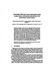
2. MATERIALS We used 10 labeled CT mediastinal lymph node VOIs (volumes-of-interest, i.e., 91x91x91 voxels centered at the annotated lymph node core position) from 5 patients with intravenous contrast; size ranges from 11.6mm to 33.6mm, to develop and evaluate the proposed method. Seven of these were used for training and the remaining three were used for testing. 2.1 Sampling and Randomness Forest training starts with the random subsampling of labeled voxels from the training volumes. Positive voxels were sampled at a rate of 60% and negative voxels were sampled adaptively. All negative voxels within 2 voxels distance from the boundary of the labeled lymph node volume were not used for training as there is low confidence of them being truly negative. They are close enough to the positive labeling mask that there may be moderate lymph node masking uncertainty. The labels of these boundary voxels have a higher chance of being mislabeled due to human error as the lymph node boundaries in the image may be indistinct. Negatives beyond 2 voxels but within 5 voxels away from the boundary voxels were randomly sampled at 40%. These negatives formed a closer shell around the labeled lymph node and are expected to provide more meaningful shape information during training due to their proximity to the image mask boundary. The remaining negatives in the training VOIs were subsampled at a lower rate (10%) as they provide only distant spatial context and thus contribute little information of the shape of the lymph node volume. The reason for this is due to the nature of the features the classifier is trained on (described in detail below and in Figure 1), the bulk of these being based on the difference in intensity between two randomly selected voxels located within a certain distance from each other. Each tree was trained on a randomly sampled subset of the training voxels that consisted of 30-50% of the total number. This data bootstrapping or sub-sampling procedure ensures the randomness of the decision trees obtained from training3.

2.2 Random Image Features and Training As shown in Figure 1 below, three types of image features were exploited: simple intensity (type I), the difference of intensity between the sampled voxel and its randomly offset voxel (type II), and the difference of two randomly offset voxels (type III). The feature space is enormously large for modeling capacity and any single image feature can be computed in O(1) time, which is highly desired. Features were selected by maximizing the information gain function. This process involved generating 500 random features, and for each feature, up to 2000 thresholds were randomly generated. The feature types are also generated from a set distribution. These thresholds were further pruned to remove redundant or insignificant thresholds – the relative difference among consecutive thresholds (of intensity for type I or difference of a pair of intensities for types II, III) should be at least 10 or above. Next, the information gain by conditional entropy of the feature for each of the remaining candidate thresholds was calculated, and the threshold that provides the highest information gain was selected for the feature.

Figure 1. Figure showing the negative voxel sampling zones and the three types of features used to construct the decision trees of the random forest. Top Left: the four sampling zones - blue indicates positive voxels to sample, green is the close negative zone, and red is the boundary zone, which is not sampled from. The remaining space is the far negative zone that is sampled at a much lower rate. Top Right: voxels selected after subsampling (different image from the top left). Red voxels are the sampled negatives and blue are sampled positives. Bottom Left: Single intensity feature (type I), only takes into account the intensity of the voxel in the original image. Bottom Center: 1- Offset feature (type II), considers the intensity difference between the selected voxel and another voxel found by randomly offsetting the original voxel. Bottom Right: 2Offset feature (type III), considers the intensity difference between two voxels, each of which is found by randomly offsetting the original voxel. The type II and type III features provide contextual information that can be used in classifying boundaries, whereas the type I features classify broader sections of the images. In the bottom three figures, the red rectangle indicates the original voxel, where the blue rectangles indicate offset voxels. The filled green rectangles are the voxels used in the feature.

Finally, each feature was compared with all other features to find the one with the highest information gain. If the maximum information gain was below a predetermined threshold or zero, or if the sample size was below a certain amount or the maximum tree depth has been reached, training terminates at this branch and the node was made a leaf. These constraints are there to prevent over-fitting of the tree, as continuing to add decision nodes to the tree when a comparatively small fraction of the samples reach this node or the samples are already quite uniform in class distribution

causes the tree to learn the exact classification of the training data, which may be slightly different from other unlabeled data that the fully trained tree may encounter in the future. Such rigid sensitivity to the training set may cause the classifier to misclassify the unseen data. The training samples at the node were split according to the feature response threshold and training proceeded recursively on the resulting left and right child nodes. Once recursion terminates, each of the leaf nodes of the decision tree contains a subset of the labeled samples. The class represented by each leaf will be determined by the number of samples of each class that reach the leaf. 2.3 Detection Testing Once trained, the forest was then applied on the testing samples. Each sample is pushed through the tree starting at the root, and the path taken depended on the sample’s feature response and the feature threshold at the internal question node learned during training. All samples ended up at a tree leaf node with a probability function that represents the likelihood of the voxel being one of two classes: either the voxel is part of a lymph node or it is not. Although we only use two classes here, this technique can be easily extended to work with multiple classes (for segmenting many organs/tissues simultaneously). The probability function derived is essentially a class histogram of the labeled training data samples that reached the leaf during training. The testing point reaches different leaf nodes in each tree of the forest, and the posterior probabilities collected at each leaf are then averaged to determine the final distribution to be used to classify the voxel.

Figure 2. Axial slices of some selected results of the classification algorithm. Images with green show the images as labelled by our algorithm, whereas images with blue show the ground truth that was manually labelled. The three pairs on the left show good classification for these particular slices of the image, but on the right there are noticeable artifacts. These might possibly be handled by finding the largest connected component to filter out smaller components that represent noise. Some poor results were expected due to the small amount of labelled training data available. The results on the middle and top right shows that the program correctly identified the area of the ground truth lymph node, but both introduced extra sections not part of the main lymph node body. It may be possible to prune these with a connected component algorithm. The bottom right result shows heavy bleeding of the label into the surrounding tissue.

2.4 Implementation Details To implement the random forest algorithm we used the Microsoft Sherwood 18,19 package for random forests. The implementation consists of several subprograms whose outputs can be linked together to construct and save a random forest data structure, which then can be loaded and applied to unlabeled data. We use separate programs to generate appropriate training and testing sets. The training subprogram subsamples both the positively and negatively labeled voxels of a subset of the 10 volumes used (in this case we used 7 volumes for constructing training data sets). The voxels of the remaining volumes are used to construct the testing set to evaluate the performance of the classifiers, which is just the set of all unlabeled voxels in the volumes. The training set generation is randomized, and different runs with different parameters will produce unique sets on which to train the forest. These training sets are fed into the forest trainer, which produces the random forest file as output. The forest file is then taken together with the testing data set and fed into a final program which applies the forest to the unlabeled testing data set, the output of which is a set of volumes labeled by the forest.

3. RESULTS Results showed promise in identifying lymph node voxels. Most lymph node voxels were effectively localized by the labeling program although there were still many small noise artifacts and bleeding into surrounding tissue. These small noise artifacts are common and can be pruned by first running a 3D connected component algorithm for grouping components and then only keeping the component with the maximal summed probability. Figure 2 shows some selected 2D axial slices of the labeled results. Some of these show great success in finding the shape of the lymph node, but others demonstrate poor segmentation performance. Figure 3 shows 3D rendered volumes of some selected results. Only those voxels that had a positive lymph node class probability of greater than 70% were labeled. The lower right example still shows a fairly large artifact that would be removed by the aforementioned post-processing.

Figure 3. 3D visualization of selected results. Green is the result labelled by the algorithm, and blue is the ground truth.

All three types of image features were randomly chosen for evaluation at 40%, 30% and 30% splitting. Nevertheless, after the intrinsic feature selection process by random forest, only 11% of the features selected were type I features in the encoded decision tree, with 35% for type II and 54% for type III features. This difference is due to the fact that although a feature of a given type may be generated during the training phase at a specific rate, the rate at which a feature type is chosen over other types for maximum information gain need not be the same. In this case, we observe that although we are generating many Type I features, few of these are being chosen as the feature that provides the highest information gain. This indicates that contextual features may be more important than intensity features in distinguishing the lymph node from surrounding tissue. We also evaluate the performance versus the tree depth. Using tree depths of above 10

introduced the problem of over-fitting, in which the forest becomes so well trained on the training data set that it degrades significantly to produce inaccurate labeling for unseen data. This is shown in Figure 4 (Top Right) by the sudden decrease in sensitivity at depth 10. This could be improved with more training data. AUCs (area under curve) of the training and validation ROC (receiver operating characteristic) curves (without over-fitting at the depth of 8) were 0.972 and 0.959, respectively. We can similarly achieve >95% sensitivity at 94% specificity to choose the operating point in ROC curve. The time it takes to train the trees is dependent on the size of training set constructed, which is in turn influenced by the subsampling rates used to select training voxels. Deeper decision trees, larger forests and a higher amount of candidate features to optimize also increase the running time of the training phase, and typical times ranged from less than five minutes to over half an hour. Note that the time spent training never needs to be repeated once the forest is finished, and much of the time cost could be optimized by implementing parallel programming methods for training multiple trees at the same time. The application of the random forests to the testing set took much less time. The running speed of the voxel labeling of each VOI is usually within a few seconds using an Intel Xeon PC.

Figure 4. Analysis of random forest performance against parameter settings. Top Left: Performance results of increasing the number of trees in the forest. Note that sensitivity improves as the number of trees increases, indicating that increasing the number of trees improves sensitivity. Top Right: Performance as a function of tree depth. As the depth increases, sensitivity decreases, a possible indication that the decision trees are over-fitting to the training data and thus less able to correctly classify the training data. Bottom Left: ROC curve for a forest of tree depth 12. Bottom Right: ROC curve for a forest that was purposely over-fitted by training on all 10 data sets and then tested on all 10 sets as well. This serves to show a theoretical upper boundary for performance.

4. CONCLUSIONS We have developed and evaluated the method using random forest and efficient image features to automatically segment lymph nodes from CT images. To the best of our knowledge, this is the first work of using random forest for lymph node voxel labeling based segmentation. Initial results show some promising performance. Most of the images labeled by the forests showed the general shape of the ground truth lymph node in the segmentation. Future work would incorporate post-processing to reduce false positives to obtain a more accurately labeled volume as well as extending the training set used to construct the random forest to use more annotated lymph node VOIs (~200). Future iterations will also use more sophisticated feature sets that take the neighborhood of each voxel into greater account. One example would be a feature that averages the intensity of all voxels within a specified range from a selected voxel, which could be accomplished in constant time if integral images are used.

ACKNOWLEDGMENTS This work was supported by the Intramural Research Program of the NIH Clinical Center.

REFERENCES [1] Breiman, L., “Random forests," Machine Learning 45(1), 5-32 (2001). [2] Lepetit, V. and Fua, P., “Keypoint recognition using randomized trees," Pattern Analysis and Machine Intelligence, IEEE Transactions on 28(9), 1465-479 (2006). [3] Amit, Y. and Y, D. G., “Shape quantization and recognition with randomized trees," Neural Computation 9, 15451588 (1997). [4] Criminisi, A., Shotton, J., and Konukoglu, E., “Decision forests: A unified framework for classification, regression, density estimation, manifold learning and semi-supervised learning," Found. Trends. Comput. Graph. Vis. 7, 81-227 (Feb. 2012). [5] Criminisi, A., Robertson, D., Konukoglu, E., Shotton, J., Pathak, S., White, S., and Siddiqui, K., “Regression forests for e_cient anatomy detection and localization in computed tomography scans," Medical Image Analysis 17(8), 1293 -1303 (2013). [6] Lempitsky, V., Verhoek, M., Noble, J., and Blake, A., “Random forest classification for automatic delineation of myocardium in real-time 3d echocardiography," in Functional Imaging and Modeling of the Heart, Ayache, N., Delingette, H., and Sermesant, M., eds., Lecture Notes in Computer Science 5528, 447-456, Springer Berlin Heidelberg (2009). [7] Yan, J., Zhuang, T., Zhao, B., and Schwartz, L. H., “Lymph node segmentation from CT images using fast marching method," Computerized Medical Imaging and Graphics 28(12), 33-38 (2004). [8] Unal, G., Slabaugh, G., Ess, A., Yezzi, A., Fang, T., Tyan, J., Requardt, M., Krieg, R., Seethamraju, R., Harisinghani, M., and Weissleder, R., “Semi-automatic lymph node segmentation in MRI," in Image Processing, 2006 IEEE International Conference on, 77-80 (2006). [9] Wang, Y. and Beichel, R., “Graph-based segmentation of lymph nodes in ct data," in Advances in Visual Computing, Bebis, G., Boyle, R., Parvin, B., Koracin, D., Chung, R., Hammound, R., Hussain, M., Kar-Han, T., Craw_s, R., Thalmann, D., Kao, D., and Avila, L., eds., Lecture Notes in Computer Science 6454, 312-321, Springer Berlin Heidelberg (2010). [10] Barbu, A., Suehling, M., Xu, X., Liu, D., Zhou, S., and Comaniciu, D., “Automatic detection and segmentation of lymph nodes from ct data," Medical Imaging, IEEE Transactions on 31(2), 240-250 (2012). [11] Barbu, A., Suehling, M., Xu, X., Liu, D., Zhou, S., and Comaniciu, D., “Automatic detection and segmentation of axillary lymph nodes," in Medical Image Computing and Computer-Assisted Intervention, MICCAI (2010), Jiang, T., Navab, N., Pluim, J., and Viergever, M., eds., Lecture Notes in Computer Science 6361, 28-36, Springer Berlin Heidelberg (2010). [12] Feuerstein, M., Deguchi, D., and et al., “Automatic mediastinal lymph node detection in chest ct." SPIE medical imaging, Computer-Aided Diagnosis, 2009.

[13] Feulner, J., Zhou, S., Huber, M., Hornegger, J., Comaniciu, D., and Cavallaro, A., “Lymph node detection in 3-d chest ct using a spatial prior probability," in Computer Vision and Pattern Recognition (CVPR), 2010 IEEE Conference on, 2926-2932 (2010). [14] Kitasaka, T., Tsujimura, Y., Nakamura, Y., Mori, K., Suenaga, Y., Ito, M., and Nawano, S., “Automated extraction of lymph nodes from 3-d abdominal ct images using 3-d minimum directional difference filter," in Medical Image Computing and Computer-Assisted Intervention MICCAI 2007, Ayache, N., Ourselin, S., and Maeder, A., eds., Lecture Notes in Computer Science 4792, 336-343, Springer Berlin Heidelberg (2007). [15] Yan, M., Lu, Y., Lu, R., Requardt, M., Moeller, T., Takahashi, S., and Barentsz, J., “Automatic detection of pelvic lymph nodes using multiple MR sequences," in Society of Photo-Optical Instrumentation Engineers (SPIE) Conference Series, 6514 (2007). [16] Dornheim, J., Seim, H., Preim, B., Hertel, I., and Strauss, G., “Segmentation of neck lymph nodes in CT datasets with stable 3d mass-spring models: Segmentation of neck lymph nodes," Academic Radiology 14(11), 1389 -1399 (2007). [17] Lu, K. and Higgins, W. E., “Segmentation of the central-chest lymph nodes in 3d MDCT images”, Computers in Biology and Medicine 41(9), 780- 789 (2011). [18] Criminisi, A. and Shotton, J., “Decision Forests in Computer Vision and Medical Image Analysis”, Springer. (2013). ISBN 978-1-4471-4928-6. [19] http://research.microsoft.com/en-us/downloads/52d5b9c3-a638-42a1-94a5-d549e2251728/ [20] Lu, L., Barbu A., Wolf, M., Liang, J., Salganicoff, M., Comaniciu D., “Accurate polyp segmentation for 3D CT colongraphy using multi-staged probabilistic binary learning and compositional model”. IEEE conference on Computer Vision and Pattern Recognition, 2008. [21] Lu, L., Bi, J., Wolf, M., Salganicoff, M., “Effective 3D object detection and regression using probabilistic segmentation features in CT images”. IEEE conference on Computer Vision and Pattern Recognition, 2011: 10491056.