Robust Optimization of Dynamical Systems with ...

Robust Optimization of Dynamical Systems with Correlated Random Variables using the Point Estimate Method ? Xiangzhong Xie ∗,∗∗,∗∗∗ Ulrike Krewer ∗,∗∗ Ren´ e Schenkendorf ∗,∗∗ ∗

Institute of Energy and Process Systems Engineering, Braunschweig University of Technology, 38106 Braunschweig, Germany ∗∗ Center of Pharmaceutical Engineering (PVZ), Braunschweig University of Technology, 38106 Braunschweig, Germany ∗∗∗ International Max Planck Research School (IMPRS) for Advanced Methods in Process and Systems Engineering, 39106 Magdeburg, Germany e-mail: {x.xie,u.krewer,r.schenkendorf}@tu-braunschweig.de Abstract: Robust optimization of dynamical systems requires the proper uncertainty quantification. Monte Carlo simulations and polynomial chaos expansion are frequently used methods for uncertainty quantification and have been applied to a number of problems in process design and optimization. Both methods, however, are either computationally prohibitive for robust optimization or inappropriate for correlated random variables. The aim of this study is to introduce the point estimate method for optimization of dynamical systems with correlated random variables. The point estimate method requires only a few deterministic evaluations of the analyzed process model and estimates the statistical moments for robust optimization. The derived sample points can be adapted to random variables of arbitrary distributions and correlations. The contribution of this paper consists of presenting the point estimate method for correlated random variables in the field of model-based robust process design. The performance of the method is demonstrated with a case study of a continuous tubular reactor. Keywords: robust optimization, uncertainty quantification, point estimate method, correlated model parameters 1. INTRODUCTION

the effect of correlations among the model parameters on the results of robust design.

Model-based optimization can be used to improve the performance of complex technical systems. Different methods are available and have been successfully applied to various problems (Biegler, 2010; Moles et al., 2003). However, uncertainties in the mathematical models decrease the reliability and efficiency of the model-based process design. Uncertainties can arise from the inherent randomness of dynamical systems or are due to extraneous disturbances from the environment and might be represented by uncertain model parameters. The parameter uncertainties lead to variations in the model output, and thus, the results from such optimization can be suboptimal or even misleading (Schu¨eller and Jensen, 2008). In addition, the correlations among uncertain parameters are also considered an important factor in the variation of the model outcome (Haaker and Verheijen, 2004). To confront this problem, robust optimization ideas are presented in the literature (Schu¨eller and Jensen, 2008; Telen et al., 2015). The goal of this paper is to introduce an efficient method for robust optimization in process design and to investigate

Two different approaches are frequently used for robust optimization: 1) the worst-case scenario and 2) the probability-based scenario. In the worst-case scenario, optimization is conducted only for extreme situations, and thus, non-extreme situations are also satisfied (Nagy and Braatz, 2003). However, the worst-case scenario requires solving a bi-level optimization problem which is nontrivial and might result in designs that are too conservative. Alternatively, the probability-based approach leads to singlelevel optimization problems and can control the robustness of constraints by changing the tolerance factors to prevent too conservative solutions (Xie et al., 2017; Telen et al., 2015). Due to these advantages, the probability-based approach is used in the current paper.

? Financial support of Promotionsprogramm “µ-Props” by MWK Niedersachsen is gratefully acknowledged.

This approach requires the propagation of the parameter uncertainties through the model and quantification of the uncertainties on the model output. Traditional samplebased methods for uncertainty quantification (UQ) are Monte Carlo simulations, quasi-Monte Carlo simulations and Latin Hypercube sampling (LHS; Singhee and Rutenbar (2010)). They require only repetitive model evaluations at different sample points of the parameter space and

are easy to implement. However, these techniques require an extremely high-computational demand, especially for systems that are computationally expensive, and thus, they are not efficient for robust process design. Arbitrary polynomial chaos (aPC) proposed by Oladyshkin and Nowak (2012) is more efficient than traditional samplebased methods and can be used for correlated random variables of arbitrary distributions. To construct the basis functions for arbitrarily correlated random variables, aPC might be too cumbersome. Alternatively, to ensure the efficiency and flexibility of robust optimization, this paper presents a point estimate method (PEM) for uncertainty quantification in robust optimization of dynamical systems. This method requires a few model evaluations to estimate the variation in the model output and can be directly used for systems with correlated parameters through a proper transformation step (Schenkendorf, 2014a; Lerner, 2002).

The approach leads to the following robust optimization problem for nonlinear dynamical systems associated with probabilistic uncertainties.

The remainder of this paper is organized as follows. Problems for robust optimization of a system with correlated random variables are formulated in Sec. 2. The PEM and the algorithm for the probability density transformation are presented in Sec. 3. The performance of the proposed method is demonstrated with a case study of a continuous tubular reactor in Sec 4. In Sec. 5, the conclusions of the paper are given.

umin ≤ u ≤ umax , (3h) where E[·] and Var[·] denote the mean and the variance values of random variables, M is the objective function of the states at tf , α denotes a scalar weight factor, [umin ,umax ] are the upper and lower boundaries for the control input vector, Pr denotes the probability of an event, hnq and hq are functions for inequality and equality constraints, and εnq , εq,µ and εq,δ are tolerance factors (Rangavajhala et al., 2009). The individual chance constraint in (3e) is approximated with the CantelliChebyshev inequality with a scalar weight factor β (Telen et al., 2015) as E[hnq ] + βVar[hnq ]0.5 ≤ 0. (4) The robust optimization framework can reduce the influence of the random variables on the optimization outcome. This is because of the following reasons. First, by optimizing the mean and the variance of the objective function, the average performance is increased, and its variation is decreased. Second, by considering the chance constraints in (4) and the approximated equality constraints in (3f) and (3g), the constraint violation tolerance and the size of design space is balanced properly.

2. PROBLEM FORMULATION Nonlinear dynamical systems can be described by different algebraic equations (DAEs) as x˙ d (t) = gd (x(t), u(t), p),

xd (0) = x0 ,

(1)

0 = ga (x(t), u(t), p) , (2) nu where t ∈ [0, tf ] is the time, u ∈ R denotes the control input vector, and p ∈ Rnp denotes the time-invariant parameter vector. x = [xd , xa ] ∈ Rnx is the state vector, in which xd ∈ Rnxd and xa ∈ Rnxa are the differential and algebra states, respectively. x0 is the vector of the initial conditions. gd and ga denote the differential and algebraic vector fields of the system. Note that t could also be the residence time which denotes the spatial coordinate related to the flow velocity in continuous processes. The dynamical system described in (1) and (2) is affected by uncertainties in the time-invariant model parameters p and initial conditions x0 . The probability space (Ω, F, P ) is defined by the sample space Ω, σ-algebra F and probability measure P . θ = [p(ω), x0 (ω)] is considered the vector of random input variables, which are functions of ω ∈ Ω on the probability space and associated with continuous probability density functions (PDFs) f (θ) = [f1 (θ1 ), . . . , fnθ (θnθ )] and the correlation matrix Σ. The first challenge of robust optimization is to incorporate the stochastic properties of the random variables into the dynamic optimization. The randomness of the system results because of the random variables can lead to strong deviations in the performance of the objective functions and may cause violations of the target constraints. To solve this problem, the objective function and constraints are characterized by their mean values and variances (Telen et al., 2015).

Problem 1 (Robust optimization with chance constraints for dynamical systems) (3a) min E[M (xtf (ω))] + αVar[M (xtf (ω))], u(t)

subject to: x˙ d (t, ω) = gd (x(t, ω), u(t), p(ω)),

(3b)

0 = ga (x(t, ω), u(t), p(ω)),

(3c)

xd (0, ω) = x0 (ω),

(3d)

Pr[hnq (x(t, ω), u(t), p(ω)) ≥ 0] ≤ εnq ,

(3e)

|E[hq (x(t, ω), u(t), p(ω))]| ≤ εq,µ ,

(3f)

Var[hq (x(t, ω), u(t), p(ω))] ≤ εq,δ ,

(3g)

The statistical moments required to solve Problem 1, i.e., E[·] and Var[·] for the state vector x, are calculated with Z xf (θ)dθ, (5) E[x] = Iθ Z (x − E[x])(x − E[x])T f (θ)dθ, (6) Var[x] = Iθ

where Iθ denotes the support of the random vector θ. Here, we have the second challenge which is to derive the joint distribution f (θ) from f (θ) and Σ. The Gaussian copula that is based on the Sklars theorem (Nelsen, 2007) is used to express f (θ) from f (θ) and Σ as follows Problem 2 (Correlated random variables) ∂ nθ Fnθ [F −1 (µ1 ), · · · , F −1 (µnθ ); Σ] f (θ) = (7) ∂θ1 · · · θnθ in which F −1 denotes the inverse cumulative distribution function (CDF) of the standard normal distribution; Fnθ denotes the joint CDF of nθ standard normal distributions with the correlation matrix Σ; and [µ1 , · · · , µnθ ] =

[F1 (θ1 ), . . . , Fnθ (θnθ )] is the CDF of θ which could be any arbitrary distribution.

can be obtained by permutations and sign changing of point ϑ = (ϑ1 , · · · , ϑr , 0, · · · , 0) ∈ Rd (r ≤ d)

The key issue for solving Problem 1 is to efficiently calculate the statistical moments given in (5) and (6). Thus, we introduce the PEM to estimate the mean and the variance of the simulation results efficiently. To solve Problem 2, we provide a sample-based algorithm that incorporates parameter correlations in Problem 1.

The generator defined in Definition 1 describes how sample points are determined deterministically. For instance, the samples used in Fig. 1 are generated with GF[0],GF[±ϑ],GF[±ϑ, ±ϑ] in R2 . Note that for GF[·] in Rd , we get 1 point from GF[0], 2d points from GF[±ϑ] and 2d(d − 1) points from GF[±ϑ, ±ϑ], which sums up to 2d2 + 1 points. Based on the derived sample points, the general approximation scheme of the PEM reads as follows (Lerner, 2002) Z k(ξ)f (ξ)dξ ≈

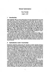
3. POINT ESTIMATE METHOD FOR CORRELATED RANDOM VARIABLES Traditional sample-based methods, i.e., Monte Carlo simulations and Gaussian quadrature, are used to calculate the high-dimensional integral terms in (5) and (6). However, their applicability is limited because of the so-called curse of dimensionality. The PEM, which requires fewer sample points in Rnθ , is a more efficient alternative method for calculating these high-dimensional integral terms with a manageable number of deterministic sample points. 3.1 Point Estimate Method Fig. 1 illustrates the principle of the PEM applied to a nonlinear function k(·) with two random inputs ξ and output variables y. Assuming a bivariate Gaussian PDF ξ ∼ N (0, I), which is symmetric and independent, the nonlinear function is evaluated at 9 dedicated sample points first, i.e., the cross, circle and star points in Fig. 1. Second, the integral term can be approximated by a weighted superposition of these function evaluations according to Z np X wi k(ξ si ), (8) k(ξ)f (ξ)dξ ≈ Iξ

i=1

ξ si

where denotes the sample points; nξ and np denote the number of random inputs and sample points, which are equal to 2 and 9 in this example; wi are the scalar weight factors and f (ξ) is the PDF of the random inputs. As we can see, the key problem in using the PEM is to find the position of the dedicated sample points and their corresponding weights.

Iξ

X

X

k(GF [±ϑ, ±ϑ]). (9) The scaling value ϑ and scalar weight factors w0 , w1 and w2 can be determined by considering low-order monomials k(ξ) = 1, k(ξ) = ξi2 , k(ξ) = ξi4 , k(ξ) = ξi2 ξj62=i (i, j ∈ {1, · · · , nξ }) as follows Z 1f (ξ)dξ, (10) w0 + 2dw1 + 2d(d − 1)w2 = w0 k(GF [0]) + w1

k(GF [±ϑ]) + w2

Iξ

Z

2w1 ϑ2 + 4(d − 1)w2 ϑ2 =

ξi2 f (ξ)dξ,

(11)

ξi4 f (ξ)dξ,

(12)

ξi2 ξj62=i f (ξ)dξ.

(13)

Iξ

Z

2w1 ϑ4 + 4(d − 1)w2 ϑ4 =

Iξ 4

Z

4w2 ϑ = Iξ

Assuming a standard Gaussian distribution,√ξ ∼ N (0, I), (10) to (13) can be solved according to ϑ = 3, w0 = 1 − 4−d 1 d2 −7d 18 , w1 = 18 , w2 = 36 . We can apply these loworder monomials because of the symmetric nature of the distributions and sample points (Schenkendorf, 2014b). In principle, we can also obtain the PEM with lower or higher precision, but the proposed setting has the best trade-off between precision and computational cost (Schenkendorf, 2014a). 3.2 PEM for Correlated Random Inputs with Arbitrary Distributions

𝜉1

y1 Nonlinear function

𝐲 = 𝐤(𝝃) 𝜉2

y2

Fig. 1. Illustration of the PEM with precision of 5 for nonlinear function y = k(ξ) which has two random inputs and two random outputs, adapted from Julier and Uhlmann (1996).

The positions of the sample points and the weights for the PEM are calculated under the assumption that the random inputs follow an independent standard normal distribution. Thus, we cannot directly use them for random inputs of arbitrary and correlated PDFs. We can solve this problem by adding a transformation step between different distributions. Proposition 1. For two random inputs (θ, ξ) with arbitrary distributions and the function Φ(·) = Fθ−1 (Fξ (·)), the following relation for the integral of nonlinear function k(θ) holds Z Z k(θ)f (θ)dθ = k(Φ(ξ))f (ξ)dξ. (14) Iθ

Definition 1 (Lerner, 2002): The generator function GF[±ϑ1 , · · · , ±ϑr ] in Rd presents the set of points which

Iξ

Proof. Fθ (θ) and Fξ (ξ) are CDFs of the two random inputs. According to the inverse transformation, we have

Z

Z

objective function and constraints, and thus, the robust optimization problem can be solved efficiently.

k(θ)dFθ (θ)

k(θ)f (θ)dθ = Iθ 1

Iθ

Z =

Z0 = Iξ

Z = Iξ

k(Fθ−1 (u))du (15) k(Fθ−1 (Fξ (ξ)))dFξ (ξ) k(Fθ−1 (Fξ (ξ)))f (ξ)dξ

In this section, we apply the proposed methods to the robust optimization of a continuous jacket tubular reactor.

2

4.1 Model Description

Here, ξ is an independent standard normal distribution, and thus, the result from Proposition 1 can now be used to transform the integral with arbitrary distribution to that of the PEM. An additional function, Φ(·) = Fθ−1 (Fξ (·)), appears after the transformation. It denotes the relation between the random inputs (θ, ξ). It can also be interpreted as sample points from the PEM for ξ are transformed via Φ(·) to the corresponding points in θ which can be directly evaluated with function k(·). However, Fθ−1 (·) is the inverse joint CDF of random variables θ derived from (7) which is too complex to evaluate directly. Therefore, we introduce Algorithm 1 adapted from Lebrun and Dutfoy (2009) to transform the samples from ξ to θ. With Proposition 1 and Algorithm 1, the PEM is now available for correlated inputs with arbitrary distributions. Algorithm 1 Sampling for correlated random variables Initialization: Random variables ξ ∼ N (0, I), I ∈ Rd×d ; θ have marginal CDFs [F1 (θ1 ), . . . , Fd (θd )] and correlation matrix Σ ∈ Rd×d ; 1: Sample U = [ξ 1 , · · · , ξ N ] with size of N = 2d2 + 1 from ξ and dimension d from Generator function GF [·]; 2: Cholesky decomposition of Σ = LLT , where L is a lower triangular matrix; 3: Correlate the sample, V = LU; 4: Transform into the sample of the Gaussian copula, W = [F (V1 ), · · · , F (Vd )]; 5: Transform into the sample of θ, M = [F1−1 (W1 ), · · · , Fd−1 (Wd )]. Technically, the mean and variance of the random variables in (5) and (6) can be estimated as E[x] = w0 x0 + w1

2nθ X i=1

xi + w2

xi ,

(16)

i=2nθ +1

(17)

i=1 2n2θ

X

Considering a tubular reactor, where an irreversible exothermic first-order reaction with reactant A and products B and C takes place according to A→ − B + C. (18) In order to control the temperature of the reactor, we supply or remove the heat by a surrounding jacket. Assuming steady state operation, a plug flow reactor model with variation only along the horizontal coordinate is adapted to describe the system. The model consists of two coupled ordinary differential equations (ODEs) which describe mass and energy conversations (Logist et al., 2008) γTn dCn αkin = (1 − Cn )e 1+Tn (19) dz v γTn βh dTn αkin δ = (1 − Cn )e 1+Tn + (u − Tn ). (20) dz v v Equations (19) and (20) are given in dimensionless form with boundary conditions of [Cn (0), Tn (0)] = [0, 0]. z is a dimensionless coordinate. Cn is the conversion of reactant A. αkin , γ, δ, βh and v are the model parameters related to the kinetic and thermodynamic constants. Tn = (Tr − Tin )/Tin and u = (Tj − Tin )/Tin are dimensionless expressions of reactor temperature Tr and jacket temperature Tj . Tin is the temperature of the inlet flow. Details regarding the model and its parameters can be found in Logist et al. (2008).

Reactor temperature Tr is bounded with an upper limit of 400 K. As the control variable, we use the jacket temperature bounded between 280 K and 400 K. For the sake of simplicity, we consider the uncertainties of two model parameters which are described by a bivariate normal distribution with αkin ∼ N (0.0581, 0.005812 )andβh ∼ 1 ρ . N (0.2, 0.022 ) and the correlation matrix Σ = ρ 1

2

2nθ X

Var[x] = w0 (x0 − E[x])(x0 − E[x])T + 2nθ X (xi − E[x])(xi − E[x])T + w1

w2

4. CASE STUDY: A CONTINUOUS JACKET TUBULAR REACTOR

(xi − E[x])(xi − E[x])T ,

i=2nθ +1

where xi is the state vector evaluated with θ i . θ i is the ith deterministic point from the sample of θ. Note that we have to solve (1) and (2) only once to get xi as point θ i is fixed for the same distribution. By this analogy, the same formula in (16) and (17) can be derived for the

The robust process design strategy aims to make a tradeoff between maximizing the conversion of reactant A while minimizing its variation because of the uncertain model parameters. The robustness of the inequality constraint of the reactor temperature is controlled by the scaling parameter β of (4). Here, β is set to 2.58 which, assuming a normal distribution, satisfies 99% of the realizations. The jacket temperature is discretized into 25 equidistant control elements. To investigate the effect of the parameter correlation, different scenarios are analyzed. The parameter correlation ρ is set to be 0, 0.8 and -0.8, which presents independent, positive and negative correlated parameters. For each correlation scenario, 9 deterministic sample points are generated according to the PEM and Algorithm 1 and are evaluated for the robust process design. All simulations are carried out in Matlab R2016a.

4.2 Results of Robust Process Design First, the underlying robust optimization problem is solved for independent random parameters with ρ = 0. The control profiles are implemented for the three correlation scenarios (ρ = 0, 0.8, −0.8) on the reactor. The resulting PDFs of the conversion of reactant A are shown in Fig. 2. Depending on the parameter correlation, we can see some variation in the distributions. In Fig. 3, we summarize the corresponding temperature profiles. The blue thick lines denote the predicted mean, and the blue dashed lines represent the 99% confidence intervals of the reactor temperature. The gray curves are 5,000 realizations of the temperature profiles depending on 5,000 parameter realizations. In Fig. 3a, the predicted 99% confidence interval perfectly satisfies the constraint, and thus, the majority of the realizations remain in the safe region. The statistics derived with the PEM are sufficient for the robust process design. However, the performance of the robust process design decreases when parameter correlations are present but are ignored during the process design phase. In this case, the target constraint is not fulfilled for a number of temperature profiles as indicated in Figs. 3b and 3c illustrating the effect of positive and negative parameter correlation. The parameter correlations have a strong impact on UQ and robust process design, respectively. To address the parameter correlations, they have to be directly considered in the process design step. In doing so, the robust optimization is solved for the reactor with ρ = 0.8 and ρ = −0.8 , respectively. In Fig. 4, we show the resulting temperature profiles. In this case, the target constraint is fulfilled reliably. The corresponding control profiles of the three correlation scenarios are presented in Fig. 5. Depending on the parameter correlation, the control profiles have significant differences especially in the range z = [0.2, 0.8].

(a) ρ = 0

(b) ρ = 0.8

60 50

PDF [-]

40 30

;=0 ; = 0.8 ; = -0.8

(c) ρ = −0.8

20 10 0 0.9

0.92

0.94

0.96

0.98

1

Conversion [-]

Fig. 2. Probability distribution functions of the conversion of reactant A at z = 1 for ρ = 0, 0.8 and −0.8. The control profile designed for ρ = 0 is used for the three parameter correlation scenarios. 5. CONCLUSION In this paper, we demonstrated the effect of parameter correlation on the results of robust optimization and process design, respectively. The point estimated method in combination with an additional transformation step are introduced to address correlated model parameter uncertainties efficiently. We analyzed the correlation effect on the

Fig. 3. Different temperature profiles with the mean values and the 99% confidence intervals for 3 parameter correlations ρ = 0, 0.8 and −0.8. The gray lines are 5,000 random realizations at different parameter combinations. The same control profile is used for all the three cases, i.e., ignoring parameter correlations. process design outcome and concluded that neglecting parameter correlations leads to non-robust designs. The case study of the tubular reactor successfully demonstrated the efficiency of the proposed concept of robust process design in the presence of parameter correlations. As a result, control profiles accounting for parameter correlations fulfilled the given process constraints reliably. Therefore, it is necessary to consider the parameter correlations for robust optimization of dynamical systems. This work also reveals prospect of the PEM as an efficient and accurate method for robust process design or other UQ-based analysis. In

(a) ρ = 0.8

(b) ρ = −0.8

Fig. 4. Correlation corrected temperature profiles with the mean values and the 99% confidence intervals for 2 parameter correlations ρ = 0.8 and −0.8 for the jacket tubular reactor. The gray lines are 5,000 random realizations at different parameter combinations.

Jacket Temperature [K]

400 380 360 ;=0 ; = 0.8 ; = -0.8

340 320 300 280 0

0.2

0.4

0.6

0.8

1

z [-]

Fig. 5. Control profiles designed for random variables with correlation factors of 0, 0.8 and -0.8. future work, we are interested in applying the methods to more complex problems and analyzing the effect of parameter correlations on robust process design in more detail. REFERENCES Biegler, L.T. (2010). Nonlinear programming: concepts, algorithms, and applications to chemical processes. SIAM. Haaker, M. and Verheijen, P. (2004). Local and global sensitivity analysis for a reactor design with parameter

uncertainty. Chemical Engineering Research and Design, 82(5), 591–598. Julier, S.J. and Uhlmann, J.K. (1996). A general method for approximating nonlinear transformations of probability distributions. Technical report, Technical report, Robotics Research Group, Department of Engineering Science, University of Oxford. Lebrun, R. and Dutfoy, A. (2009). A generalization of the nataf transformation to distributions with elliptical copula. Probabilistic Engineering Mechanics, 24(2), 172–178. Lerner, U.N. (2002). Hybrid Bayesian networks for reasoning about complex systems. Ph.D. thesis, stanford university Stanford, CA. Logist, F., Smets, I., and Van Impe, J. (2008). Derivation of generic optimal reference temperature profiles for steady-state exothermic jacketed tubular reactors. Journal of Process Control, 18(1), 92–104. Moles, C.G., Mendes, P., and Banga, J.R. (2003). Parameter estimation in biochemical pathways: a comparison of global optimization methods. Genome research, 13(11), 2467–2474. Nagy, Z.K. and Braatz, R.D. (2003). Worst-case and distributional robustness analysis of finite-time control trajectories for nonlinear distributed parameter systems. IEEE Transactions on Control Systems Technology, 11(5), 694–704. Nelsen, R.B. (2007). An introduction to copulas. Springer Science & Business Media. Oladyshkin, S. and Nowak, W. (2012). Data-driven uncertainty quantification using the arbitrary polynomial chaos expansion. Reliability Engineering & System Safety, 106, 179–190. Rangavajhala, S., Mullur, A.A., and Messac, A. (2009). Equality constraints in multiobjective robust design optimization: Decision making problem. Journal of optimization theory and applications, 140(2), 315–337. Schenkendorf, R. (2014a). A general framework for uncertainty propagation based on point estimate methods. In Second European Conference of the Prognostics and Health Management Society, PHME14, Nantes, France. Schenkendorf, R. (2014b). Optimal experimental design for paramter identification and model selection. Ph.D. thesis, Otto-von-Guericke-Universit¨at Magdeburg. Schu¨eller, G.I. and Jensen, H.A. (2008). Computational methods in optimization considering uncertainties–an overview. Computer Methods in Applied Mechanics and Engineering, 198(1), 2–13. Singhee, A. and Rutenbar, R.A. (2010). Why quasi-monte carlo is better than monte carlo or latin hypercube sampling for statistical circuit analysis. IEEE Transactions on Computer-Aided Design of Integrated Circuits and Systems, 29(11), 1763–1776. Telen, D., Vallerio, M., Cabianca, L., Houska, B., Van Impe, J., and Logist, F. (2015). Approximate robust optimization of nonlinear systems under parametric uncertainty and process noise. Journal of Process Control, 33, 140–154. Xie, X., Schenkendorf, R., and Krewer, U. (2017). Robust design of chemical processes based on a one-shot sparse polynomial chaos expansion concept. Proceedings of the 27th European Symposium on Computer-Aided Process Engineering.