ROBUST PRECODING FOR MULTI-USER MISO ... - CiteSeerX

ROBUST PRECODING FOR MULTI-USER MISO SYSTEMS WITH LIMITED-FEEDBACK CHANNELS Paula M. Castro , Michael Joham! , Luis Castedo , and Wolfgang Utschick! ! University of A Coru˜na, Campus de Elvi˜na s/n, A Coru˜na, Spain, 15071 Email: pcastro,[email protected] "! Munich University of Technology, Theresienstr. 90, 80290 Munich, Germany Email: joham,[email protected] ABSTRACT In Multi User Multiple Input Single Output (MU-MISO) systems one centralized transmitter with multiple antennas serves several decentralized single-antenna receivers. Precoding is an attractive way to remove multiuser interferences because it reduces cost and power consumption in the user equipment. When implementing precoding, however, the base station should know the Channel State Information (CSI). In Frequency Division Duplex (FDD), this information is sent from the receivers by means of a feedback channel, whose data rate is often severely limited. In this paper we investigate the utilization of the Karhunen-Lo`eve (KL) transform to compress the CSI sent through the feedback channel. We model the errors caused by channel estimation, truncation and quantization of the KL coefficients and feedback delay. This error modeling is the basic premise to design robust Tomlinson Harashima Precoding (THP) based on a sum Mean Square Error (MSE) criterion. Our results show that robust THP clearly outperforms conventional THP transmitting a minimum amount of information from the receivers. 1. INTRODUCTION Dirty Paper Coding (DPC) [1] combined with a Signal-toInterference-plus-Noise Ratio (SINR) criterion [2, 3] is an attractive signaling scheme for the downlink of Multi User Multiple Input Single Output (MU-MISO) systems. This is a point-to-multipoint channel which is referred to as broadcast channel in information theory [4]. In this work we focus on a low-cost and straightforward way to implement DPC, namely, Tomlinson-Harashima Precoding (THP) [5,6]. THP is suboptimal compared to DPC and suffers from shaping and modulo loss due to the modulo operations at the transmitter and the receivers [7]. As shown in [8], the SINR and the Mean Square Error (MSE) achievable regions for MU-MISO systems are The authors would like to thank by the support of this work, under grants number PGIDT05PXIC10502PN and TEC2004-06451-C05-01, to Xunta de Galicia, Ministerio de Educaci´on y Ciencia of Spain and FEDER funds of the European Union.

tightly related. Therefore, it is not surprising that the suboptimal sum MSE design of [9, 10] shows an excellent performance. The design of DPC systems is already known for the ideal case where Channel State Information (CSI) at the transmitter is perfectly known. However, the situation is different for the case with erroneous CSI, where no scheme comparable to that of [1] has been proposed nor the capacity region has been found yet. Additionally, the application of the SINR criterion is questionable, since it is unclear up to now how to include the uncertainties in the SINR in a systematic way (see the discussion in [11] and the attempt in [12] for the case of statistical CSI). Consequently, it is inevitable to resort to an MSE criterion together with THP for the case of partial CSI, since a THP design based on the sum MSE criterion is possible, as demonstrated in [13, 14]. Most work on precoding with erroneous CSI has mainly focused on Time Division Duplex (TDD) systems. Contrarily, in this work we focus on the more extended case of Frequency Division Duplex (FDD) systems where the transmitter cannot obtain the CSI from the received signals, even under the assumption of perfect calibration, because the channels are not reciprocal. Instead, the receivers estimate their channels and send the CSI back to the transmitter by means of a feedback channel. This is a reasonable assumption since currently standardized wireless systems have control channels to implement adaptive transmit facilities such as power control or adaptive modulation. Since the data rate of the feedback channels is often limited [15], the CSI must be compressed to ensure that the tight scheduling constraints are satisfied. To limit the CSI sent to the transmitter we will use in this paper a truncation of the Karhunen-Lo`eve (KL) decomposition which is optimum in the sense that it provides dimensionality reduction with the smallest possible MSE. In this work we study the following sources of errors in the proposed precoding design: channel estimation, truncation of the KL transform, quantization of the KL coefficients, and feedback channel delay. With the obtained error model, we develop robust THP that takes into account the statistical

$ "

#

"!

#! precoding

"!

& ! '%

"

.

!

.. .

.. .

#

$!"

!!

properties of the errors in the fed back CSI. Our simulation results show that using robust THP designs a considerable compression rate is possible without sacrificing performance. This paper is organized as follows. Sections 2 and 3 describe the signal and channel models, respectively, and in Section 4, the models for the CSI error sources are developed. Section 5 presents our robust THP design. Illustrative computer simulations are presented in Section 6 and some concluding remarks are made in Section 7.

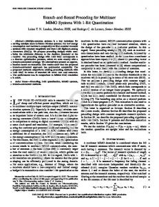
We consider a MU-MISO system with t transmit antennas and single antenna receivers as depicted in the Fig. 1. The precoder generates the transmit signal from all data symbols ! belonging to the different users . The signal ! from transmit antenna propagates over the channel with the coefficient "#! to the -th receiver, superimposes with the signals of the other transmit antennas, and is perturbed by the additive white Gaussian noise " with variance $! , i.e.,

# $ $ $# !

(

)

*

+" !

%

t

!"

'"#!%! " )" ! !#"

" )"

(1)

' # $ $ $# '

where #"$# denotes transpose and !" ! % "# "#%t ℄# # %t represents the flat fading vector channel corresponding to the -th user. Figure 2 plots the block diagram of a MU-MISO system with THP. As you can see in the figure, the received signal " is then multiplied by a common gain factor that acts as an automatic gain control. In THP, a modulo operator is applied to the weighted received signal to remove the ambiguities introduced by the precoder (see e.g., [16]). The resulting estimate of " is denoted by '" . At the transmitter, the feedforward filter " $ suppresses parts of the interference linearly, whereas the feedback loop with the strictly lower triangular feedback filter # $ $ $ subtracts the remaining interferences non-linearly. Note that #"$$ indicates conjugate transpose. Since the order of precoding has an effect on performance, the data signal % is reordered

(

,-

"

"

#.

!

by means of the permutation filter ' ! &" (& (# "! , where (& is the -th column of the & identity matrix and & is the index of the -th data stream to be precoded [10]. The signal ' % is passed through the feedback loop:

.

+

.

! !

" "

##

& ! % ' % $ #$ $ $ &

(

(2)

where the modulo operator %#"$ limits the amplitude of & and thus, the power of the transmit signal . Additionally, the entries of & have statistical properties which approximately only depend on the modulo constant (see e.g., [7]). In particular, %&& $ ℄ ! '! $ with '! ! ! *. The output & of the feedback loop can alternatively be computed with the pseudo code in Table 1. The signal & is transformed by the feedforward filter " $ to get the transmit signal , which must satisfy an average total transmit power constraint, i.e., %' # $'!! ℄ ! tr .

0

0

2. SYSTEM MODEL

&

.

data.

channels.

'

.

Table 1. Computing the feedback loop output from the permuted !

Fig. 1. Multiuser system model with precoding over flat MISO

! " #$$$#" %

# $ $ $# !

for ! &# $ ! %#(&# $ $ # $ #) $&$ ! " $&

!

)

*

*

/

/,

0

3. CHANNEL MODEL

(

We model the -th user channel vector as a vector of zeromean circularly symmetric complex Gaussian distributed random variables, i.e.,

!" ( )

#

# )(#" $

(3)

(

where )(#" is the covariance matrix of the -th user’s channel. The channels of the different users are statistically independent. In the -th time slot, our model for the -th user channel vector is )!! # $ !" # $ ! )(#" (4) w#"

1

1

(

1

1$

with !w#" # $ being a vector of stationary circularly symmetric complex white Gaussian processes (with unit variance elements) and where #"$ )! represents the Cholesky decomposition. According to the modified Jakes model [17, 18] described in [19], temporal channel correlations are modeled by !w#" # $ whereas the spatial correlations are introduced by the )! multiplication by )(#" [20]. Notice that, according to our model, the channel !" is stationary because !w#" is stationary. Realistic channels are often non-stationary, e.g., either the location of the receiver or the scenario geometry can change. Thus, the channel covariance matrix has to be tracked in real situations. However, since the covariance matrix changes very slowly compared to the channel itself, it is realistic to assume that it is constant and perfectly known at both the receiver and the transmitter.

1

!

"

#! #

$"

!

!

!!" !

!

−

!! " #

$"

!

TX

!!" !

!

Compression Techniques

!

!"

Feedback channel

Fig. 2. Block diagram of Tomlinson-Harashima precoding. According to [20], we have that !"

#

! !" ! $ ! "!$ "!$ SF

(5)

with

!!"!$ ℄%

e#$%& %&'$'BS ! ('" )) "

#

!#" $ $ $ " %t "

(6)

!$" %'& is the angle of departure from the where &BS!" transmitter to the ( -th user, &$ (different constant values depending on the environment, see [20]) is the offset for the )-th sub-path with respect to &BS!" and SF represents the log-normal shadowing, which is ' dB for suburban macrocell [20]. In [20], the number ! of sub-paths per-path is %$.

our model considering a system without feedback delay but a delayed observation for the channel estimator. That partial CSI is then used at the transmitter to reconstruct the channel vector and to design the THP filters. In the following subsections we describe this process with more detail and obtain the statistical description of the errors incurred at each step. Along this section we will assume that the signals and errors are uncorrelated.

4.1. Statistical model for channel estimation errors (Type A) We use linear estimators at the receiver based on %tr pilot symbols per time slot * to enable the channel vector estimation for the ( -th user, i.e.,

"( " )*& #" )*&$" )*&

4. IMPERFECT CSI In realistic situations, the CSI that is available at the transmitter is not perfectly known. In this case, it is a matter of discussion what kind of information has to be sent to the transmitter and the way of recovering it from the receiver side. CSI can be obtained by different mechanisms in the receiver side which gives rise to more or less degradation in the final information sent through the feedback channel. In the system that we propose in this paper we start estimating the channel at the receivers using the observations of the pilot symbols, which requires knowledge about its covariance matrix. Then, we project the resulting channel estimation onto the eigenvectors of the channel covariance matrix to obtain the KarhunenLo`eve transformation of the channel vector which optimally provides a dimensionality reduction with the smallest possible MSE. The coefficients of the truncated KL expansion are then quantized prior to transmission over the feedback channel which introduces a delay. We incorporate this delay in

(7)

$

where " )* & reads as

$" )*& %"" )*& * &" )*& % &" )*& with

(8)

(tr (t containing the training symbols [21] and (tr ! being the AWGN with variance * . )

We use the heuristic estimator [22] so that the least-square channel estimates are obtained when we consider the estima! ) " &"! " . Therefore, the channel tor " )* & estimate is given by

#

%

% % %

"LS!" )*& %!$" )*& "" )*&* %! &)*& "" )*&* &LS!" )*&

(9)

with

&LS!" )*& # $ )

" )* )% " % &"! &$

(10)

4.2. Statistical model for Karhunen–Lo`eve errors (Type B)

#

!!" "!#!" "!#℄

!"

$!"

!

!" reads as

The eigenvalue decomposition of

""!$ ""!$ ""!$ #

" "

#

"

(11) where #" is the rank of and and " are, respec!" "!$ "!$ tively, the $-th eigenvector (or $–th column of the matrix " ) and the $-th eigenvalue of !" (or the $–th entry of the diagonal matrix " ). Applying the KL transform, the channel vector in the time slot ! can be obtained as " " "! #, where " "! # are the coefficients of the KL transform given by " "! # LS!" "! #. " No errors are added to our channel estimation if all the coefficients of the KL transform are employed. To compress the channel information and taking into account the good energy compaction properties of the KL decomposition, we can approximate the vector channels " "! # by

"

#

#



# !

! #" #" !LS!" "!# #" #" !" "!# % #" #" %LS!" "!#

!KL!" "!# #" " "!#

to the transmitter due to the fast variations of the channel (so referred as short–term variations). The uniform quantizer is the most common of the scalar quantizers whose principle is rather simple. With the normalization of the KL coefficients "!$ "! # given by "!$ "! #) "!$ , where $ denotes the $-th entry of the diagonal matrix " and of the KL coefficients vector " "! #, we get a standard Gaussian distribution for them. We can approximately assume that the input is bounded, with real and imaginary values independently # quantized#lying in the range included between &&'() ) and &&'() ), i.e., the overload region has very low probability ($ *&*+) of containing any input sample. The process of quantization is as follows. Before # transmission, # we choose representants between &&'() ) and &&'() ) to construct an initial set of codebooks that are stored at both transmitter and receiver. The receivers perform a search to find for the components (real and imaginary parts) of the KL coefficients obtained in each time slot the element in the codebook that is closest. Then, the corresponding codebook index is fed back to the transmitter. Finally, the transmitter simply looks at its codebook and builds the precoder parameters from the selected codeword [23]. Therefore, KL!" lies somewhere in the respective cell, i.e.,

!

(12)

#

"

" ! ## %

! "!" % & & & % "!# % %t %!!" ℄ and # denotes the where " number of KL coefficients sent from the receiver after truncation. The noise " " LS!" "! # and the signal " " " "! # lie in the same subspace spanned by the columns of " . Therefore, KL!" "! # gives us no information about the properties of " "! # lying in range" " #! . The resulting error contribution due to the KL truncation reads as

!

!

## ! #

#

! " "!#

"& #" #" #!" "!# ! " "!% "& #" #" #

!"

"& #" #" ##& (13)

# # %LS!" "!# is orthogonal to ! " "!#.

Note that " " So, we have

!" "!# ! " "!# % ! " "!#

!

(16)

%

where Q!" is the representant and where Q!" "! # is assumed uniformly distributed over the cell, for simplicity reasons. Even though the input is not uniform if the number of levels for uniform quantization * is large and, therefore, the quantizer step , is very small, we can assume that the input pdf is very # $ [24], where + is the error in smooth and that "%+% # "# the uniform quantizer. Remember that KL!" "! # only lies in the subspace spanned by the columns of " . Under the assumption that also the quantizer works in this subspace, i.e., Q!" "! # " Q!" "! #, we can follow that Q!" "! # lies also in the subspace spanned by the columns of " . Therefore, we get the rank deficient covariance matrix for the quantization error

!

#

!

% #

Q!"

(14)

#"

Q

#!

#"

(17)

&

with

! " "!# !KL!" "!# % %KL!" "!# and %KL!" "! # ! " "!% '&# # # "' ' #"" # # #.

!KL!" "!# !Q!" "!# % %Q!" "!#

(15)

4.3. Statistical model for quantization errors (Type C) Given that our channel covariance matrix does not depend on time [cf. (5)], the modal matrix obtained from its eigenvalue decomposition is also constant over time. With this assumption, only the KL coefficients have to be sent from the receiver

$ % % , since the KL coefficients are uncorwhere Q % t t related and consequently, the quantization errors are too, the variance is ) !%+%# ℄. Taking into account the errors due to estimation, truncation of the KL transform and quantization, we have up to now the following model

!" "!# !Q!" "!# % %Q!" "!# % %KL!" "!# % ! "!#& Note that the error covariance matrix has full rank.

Q!"

%

KL!"

%

(18) h

!"

!"

!

#Q! !KL!

!Q !

!#

Q! Q!

where and

!" !

!KL!

!#

!#

is the quantized version of "

! !

LS!

! $! ! !! ! !℄ " " " ! " " " #" $ $ ! # & ' " $ " # ! " % " " " !#$! % " " " ! ! Q !

Q

" #

$

!

!

!

"! !

%

!!

%#

& #D,k slot

&

!

!

#$! " " !

!

Table 2. The errors model. 4.4. Statistical model for feedback delay errors (Type D)

!

The transmission over the feedback channel introduces a deslots. This delay can equivalently be modeled as lay of follows. The estimator gets outdated training data, i.e., the observation of the estimator is delayed by slots. Then, the respective feedback channel has no delay. The LS estimate for delayed training data reads as LS

!"

!

!LS

#! $

!

!

!

(19)

where !LS ! ! has the same statistical properties as described above in (10). Clearly, LS

!

!

"

!

!$

!

#!

"

!

!$

!LS

!

being !LS ! ! " ! #! properties of ! ! and taking into account that

!

"

!

"w !

" "

!! !

w

!

!$

!

!LS

! ! $

(20)

$

℄

"

"

'

" !

" % w !! w !! #! '$ %%Dslot # !

!℄

!

!

#t

"

'

(

"%

(21)

#t

#! !!!℄ " % % " & #! '$ %Dslot !

!

!

!

!

!

(22)

" !

with "

"

(" % %

!

!

!"

% !!# $ '

"

(

!

"

") " " "

"

'" "

#

#! '$

$

%"

"

$"

!

!"

$#

) "

)" * "

!"

)" *

"" " *

"

! !

)$ " $

whose -th and $ -th rows are exchanged

)" *

)" * "

&

" !"

""

"

") "

)" *

)" *

$

""

#$ ! upper triangular part of " $ $ ! # , % $ ! & $ # #$ " $ " " $ " ' ! !% )*" " !" + %% !% )*" , * ! !"

"" " *

") "

"

)tr &'

% $ ! (% $

&D,k &slot

(23)

##

"

" !

5. ROBUST THP DESIGN It is very well–known that THP performance degrades strongly due to imperfect CSI at the transmitter. For a multi–user scenario we have non–cooperative receivers and, therefore, linear equalization cannot be performed at the receiver. Thus, it will be necessary to stochastically model the errors (as was made in Section 4), designing an average robust THP with it, studied for a similar application in [14]. Our model for the channel matrix is given by !" #

#!℄

!. Here $$ " ! #! ! Hence, the new LS error has the property

!LS

$!

With the ! showed in Section 3, and

%

$

! ! "###"$

!.

# %

$

$ ! #$% &'( %

Table 3. Calculation of robust THP filter with optimum ordering.

!LS

where ! denotes the zero–th order Bessel function of the first kind, D ! is the maximum Doppler frequency, and slot the slot rate, we obtain

" %$

&& ! # %%

"

!! ,"!! for ! !" # # # " "

( !

!

!

%

!.

Therefore, at the end, we find the model of the errors described in Table 2.

!$

T

!

(24)

where # ! is the quantized version of the channel matrix and T ! is the error matrix. We follow the robust design of [14], i.e., we solve a robust optimization according to our error model of the feedback channel. For the efficient THP implementation described in [10] and shown in Table 3, we start from

!

"

#

! ! #

!$

!"

T

$

%

!

"

!

(25)

with ! denoting the signal to noise ratio (SNR) that is defined as the ratio between the total transmitted energy, "tr , and the

noise spectral density, and where

T

# #"

T "! #℄

!

#"

T

"!"

(26)

−1

10

−2

10

the conjugation and where

BER

denoting "

! T "! #

0

10

#" % !" !"# ""$$ "" # " #!" &"' ! #% "&$ %%D#" &## %#" #!" !"#

T

−3

10

Q

% slot # % "# ! !" !" # %#" "# ! !" !"# #'

−4

Perfect CSI Erroneous CSI with errors type A Erroneous CSI with errors type A and D Erroneous CSI with errors type A, B, C and D

10

(27) −5

Thus, by considering the statistical properties derived for the errors in the previous section in the algorithm used to obtain the filters, we can compensate in advance the impairments of the channel state information at the transmitter side to avoid an increase of the complexity of the receiver terminals.

10 −10

−5

0

5

10 SNR in dB

15

20

25

30

Fig. 3. BER performance vs. SNR for non-robust THP and v=10 km/h.

6. SIMULATIONS 5.1. MMSE receiver equalizer Additionally, when we design the gain factors according to the Minimum Mean Square Error (MMSE) equalizer [25, 26] instead of using the modulo gain '() at the receiver side, we can improve the overall system performance with a small increase in the receivers complexity. The received signal corresponding to the * –th user is +" . The output ," of the MMSE gain factor is obtained as,

," "- .!"#+"

(28)

where . is the variance of +" and - is the cross correlation between the * -th user’s received signal +" and the desired & & # for user *. These desired symbols value /" " are obtained from the linear representation [10] of the nonlinear modulo operator at the transmitter in Fig. 2. According to (1), the values of . and - are

$% & '

! +" $"

. -

!#

!+" /" ℄

!

$

"

(&" ) # !)(" % "$$ (&" ) #' % 0" '#&%$" (29) (&" ) # !&%$" '

" "

where is a diagonal matrix corresponding to the covariance matrix of the signal and whose entries are equal to 1 $ (( except the first one that is '. Clearly, - cannot be computed from a channel estimate, because the receiver has no knowledge about the precoder # and the permutation matrix . However, the transmitter can linearly precode the symbols during the training phase such that symbols for the * -th receiver are weighted prior to transmission with # " . Consequently, the received signal corresponding to the transmitted training symbols contains the term # " 2training#" and the needed cross correlation - can be estimated.

'

)

%

) !&%$ ) !&%$

In this section, we present the results of several computer simulations that we carried out to validate the proposed system. The figures illustrate how each type of error degrades the system more and more (see Fig. 3) and how robust THP can be employed to improve the performance and compensate the channel effects when the mismatch is caused by the different error sources that have been presented in this paper. The results are the mean of )*** channel realizations and '** symbols were transmitted per channel realization. The input bits are QPSK modulated. Figures show the performance for 3t 4 +. We consider an %slot of ')** Hz at a center frequency of 2 GHz. We also consider errors due to the feedback delay, being & equal to ' for all users. The figures show the estimated BER curves for a Doppler frequency normalized to the slot period of *'*'&, (v '* km/h), i.e., relatively fast fading. Fig. 4 plots the loss in performance when KL compression is applied. It can be seen, however, that 5 & coefficients can be enough to ensure a suitable system performance with the enormous advantage of reducing the overhead of the feedback channel, especially for a high number of antennas at the transmitter. Note that a compression ratio given by &("")' , where 6 and 7 is the number of bits employed for, respectively, coding the real and imaginary part of the channel coefficients 8"#* (1) and representing the codebook index, can be reached employing only that truncation of the KL coefficients and the described quantization process prior to transmission. For example, in these simulation results, we use a codebook of '*&- (7 '*) entries and if 6 ,& bits are used to encode the real and imaginary value of each channel coefficient, we obtain in a very simple way a compression ratio of '&'+. With a reasonable codebook size, we are obtaining good performance. Obviously, larger sizes improves the performance at the cost of decreasing the compression for the CSI sent

0

10

0

10

−1

10

−2

BER

BER

10

−3

−1

10

10

−4

10

0

5

10 SNR in dB

15

20

25

30

Fig. 4. BER performance vs. SNR when only truncation of KL coefficients is applied for non-robust THP and v=10 km/h. through the feedback channel and greatly extending the storage capability necessary at the receivers [23]. The precoding performance for different user speeds is plotted in the Fig. 5. You can see the curves for a speed of !, "! and #! km/h (normalized Doppler frequency of ! ! $", ! !"%! and ! !%& , respectively). Obviously, the loss in performance for faster fading is greater than for slower fading, although with robust THP we can always get better performance with not much fed back CSI, as you can see in the figure. Thus, Fig. 6 shows the estimated BER curves when we have a macro-cell environment which determines an offset of $ degrees according to the model described in [20] and in Section 3. You can see how the non-robust THP curves go up for high SNR due to the sensitivity of our THP scheme to imperfect CSI. The figure plots the improvement in performance with respect to standard THP when the proposed robust THP scheme is applied. As you can see in the figure, the loss due to imperfect CSI can be reduced if we also apply the MMSE equalizer described in Section 5, so that the channel effects are compensated between both the transmitter and receiver side. Finally, if we have a macro-cell environment which determines an offset of "' degrees, you can see in the Fig. 7 how the performance is worse than for $ degrees, given that the environment obstructs even more the signal transmission.

−2

10 −10

−5

0

5

10 SNR in dB

15

20

25

30

Fig. 5. BER performance vs. SNR for different user speeds.

0

10

THP RTHP THP+MMSE equalizer RTHP+MMSE equalizer −1

10

BER

−5

−2

10

−3

10

−4

10 −10

−5

0

5

10 SNR in dB

15

20

25

30

Fig. 6. BER performance vs. SNR for robust and non-robust THP when an offset of deg is considered for the Spatial Channel Model.

0

10

THP RTHP THP+MMSE equalizer RTHP+MMSE equalizer

BER

−5

10 −10

THP for v=10km/h THP for v=30km/h THP for v=60km/h RTHP for v=10km/h RTHP for v=30km/h RTHP for v=60km/h

Perfect CSI Erroneous CSI with errors type B (4 coef.) Erroneous CSI with errors type B (2coef.) Erroneous CSI with errors type B (1 coef.)

7. CONCLUSION In this paper, we have demonstrated the feasibility of quantization and truncation of KL decomposition for MU–MISO Tomlinson–Harashima precoding in FDD systems. Thanks to these techniques, the feedback channel overhead is strongly reduced. We have also considered the effect of estimating the channel using supervised methods and the delay inherent to the feedback channel, so that we model these errors and design a robust THP scheme which clearly outperforms the

−1

10 −10

−5

0

5

10 SNR in dB

15

20

25

30

Fig. 7. BER performance vs. SNR for robust and non-robust THP when an offset of !" deg is considered for the Spatial Channel Model.

conventional THP design. Thus, we are capable of adapting the precoder parameters to channel variations with a limited feedback channel.

[13] A. P. Liavas. Tomlinson-Harashima Precoding With Partial Channel Knowledge. IEEE Transactions on Communications, vol. 53, no. 1, pp. 5–9, January 2005.

8. REFERENCES

[14] F. A. Dietrich, and W. Utschick. Robust Tomlinson-Harashima Precoding. In Proc. of the 16th IEEE Symposium on Personal, Indoor and Mobile Radio Communications, vol. 1, pp. 136– 140, Berlin, Germany, 2005.

[1] M. Costa, Writing on Dirty Paper. IEEE Transactions on Information Theory, vol. 29, no. 3, pp. 439–441, May 1983. [2] P. Viswanath and D. N. C. Tse, Sum Capacity of the Vector Gaussian Broadcast Channel and Uplink-Downlink Duality. IEEE Transactions on Information Theory, vol. 49, no. 8, pp. 1912–1921, August 2003. [3] M. Schubert and H. Boche, Iterative Multiuser Uplink and Downlink Beamforming Under SINR Constraints. IEEE Transactions on Signal Processing, vol. 53, no. 7, pp. 2324– 2334, July 2005. [4] T. M. Cover and J. A. Thomas. Elements of Information Theory. John Wiley & Sons, 1991. [5] M. Tomlinson. New Automatic Equalizer Employing Modulo Arithmetic. Electronic Letters, vol. 7, no. 5/6, pp. 138-139, March 1971. [6] H. Harashima and H. Miyakawa. Matched–Transmission Technique for Channels with Intersymbol Interference. IEEE Journal on Communications, vol. 20, no. 4, pp. 774-780, August 1972. [7] R. F. H. Fischer. Precoding and Signal Shaping for Digital Transmission. John Wiley & Sons, 2002. [8] M. Schubert and S. Shi. MMSE Transmit Optimization with Interference Pre-Compensation. In Proc. VTC 2005 Spring, vol. 2, pp. 845–849, May 2005. [9] M. Joham and W. Utschick. Ordered Spatial Tomlinson Harashima Precoding. In Smart Antennas — State-of-the-Art, ser. EURASIP Book Series on Signal Processing and Communications, T. Kaiser, A. Bourdoux, H. Boche, J. R. Fonollosa, J. B. Andersen, and W. Utschick, Eds., EURASIP, Hindawi Publishing Corporation, 2006, vol. 3, ch. III. Transmitter, pp. 401–422.

[15] D. J. Love, R. W. Heath Jr., W. Santipach, and M. L. Honig. What is the value of the limited feedback for MIMO channels?. IEEE Communications Magazine, vol. 42, pp. 54-59, October 2004. [16] M. Joham, D. A. Schmidt, J. Brehmer, and W. Utschick. Finite-Length MMSE Tomlinson-Harashima Precoding for Frequency Selective Vector Channels. Accepted for publication in IEEE Transactions on Signal Processing, 2006. [17] W. Jakes. Microwave Mobile Communications, New York: Wiley, 1974. [18] T. Croft, P. Dent, and G. E. Bottomley. Jakes fading model revisited. IEEE Electronics Letter, vol. 29, 1993. [19] T. Zemen. Time–Variant Channel Estimation Using Discrete Prolate Spheroidal Sequences. IEEE Trans. on Signal Processing, vol. 53, No. 9, September 2005. [20] 3rd Generation Partnership Project; Technical Specification Group Radio Access Network; Spatial channel model for Multiple Input Multiple Output (MIMO) simulations (Release 6), 2003. [21] J. Balakrishnan, M. Rupp, and H. Viswanathan. Optimal channel tracking for multiple antenna systems. In Proc. of the conference on multiaccess, mobility and teletraffic for wireless communications, December 2000. [22] F.A. Dietrich, and W. Utschick. Pilot–Assisted Channel Estimation Based on Second-Order Statistics. IEEE Trans. Signal Processing, vol. 53(3), pp. 1178-1193, March 2005. [23] P. M. Castro and L. Castedo. Adaptive Vector Quantization for precoding using blind channel prediction in frequency selective MIMO mobile channels. In Proc. ITG/IEEE Workshop on Smart Antennas 2005, April 2005.

[10] K. Kusume, M. Joham, W. Utschick, and G. Bauch. Efficient Tomlinson–Harashima Precoding for Spatial Multiplexing on Flat MIMO Channel. In Proc. ICC 2005, vol. 3, pp. 20212025, May 2005.

[24] A. Gersho and R. Gray. Vector Quantization and Signal Compression. Kluwer Academic Publishers, 1992.

[11] R. El Assir, F. A. Dietrich, M. Joham, and W. Utschick. MinMax MSE Precoding for Broadcast Channels based on Statistical Channel State Information. In Proc. SPAWC 2006, July 2006.

[26] J. G. Proakis and M. Salehi. Communication systems engineering. Prentice Hall, 1994.

[12] B. Chun. A Downlink Beamforming in Consideration of Common Pilot and Phase Mismatch. In European Conference on Circuit Theory and Design, September 2005.

[25] E. A. Lee and D. G. Messerschmitt. Digital Communication. Second Edition. Kluwer Academic Publishers, 1994.