Robust Probabilistic Filtering in Distributed Systems - Carnegie Mellon

Robust Probabilistic Filtering in Distributed Systems Stanislav Funiak, Carlos Guestrin, Mark Paskin*, Rahul Sukthankar** January 2007 CMU-ML-07-102

Robust Probabilistic Filtering in Distributed Systems Stanislav Funiak Carlos Guestrin Rahul Sukthankar∗∗

Mark Paskin∗

January 2007 CMU-ML-07-102

School of Computer Science Carnegie Mellon University Pittsburgh, PA 15213

Abstract We present a robust distributed algorithm for approximate probabilistic inference in dynamical systems, such as sensor networks and teams of mobile robots. Using assumed density filtering, the network nodes maintain a tractable representation of the belief state in a distributed fashion. At each time step, the nodes coordinate to condition this distribution on the observations made throughout the network, and to advance this estimate to the next time step. In addition, we identify a significant challenge for probabilistic inference in dynamical systems: message losses or network partitions can cause nodes to have inconsistent beliefs about the current state of the system. We address this problem by developing distributed algorithms that guarantee that nodes will reach an informative consistent distribution when communication is re-established. We present a suite of experimental results on real-world sensor data for two real sensor network deployments: one with 25 cameras and another with 54 temperature sensors.

∗

Google

∗∗

Intel Research

This research was supported by grants NSF-NeTS CNS-0625518 and CNS-0428738 NSF ITR. S. Funiak was supported by the Intel Research Scholar Program; C. Guestrin was partially supported by an Alfred P. Sloan Fellowship.

Keywords: Graphical Models; Sensor Networks

1

Introduction

Large-scale networks of sensing devices have become increasingly pervasive, with applications ranging from sensor networks and mobile robot teams to emergency response systems. Often, nodes in these networks need to perform probabilistic dynamic inference to combine a sequence of local, noisy observations into a global, joint estimate of the system state. For example, robots in a team may combine local laser range scans, collected over time, to obtain a global map of the environment; nodes in a camera network may combine a set of image sequences to recognize moving objects in a heavily cluttered scene. A simple approach to probabilistic dynamic inference is to collect the data to a central location, where the processing is performed. Yet, collecting all the observations is often impractical in large networks, especially if the nodes have a limited supply of energy and communicate over a wireless network. Instead, the nodes need to collaborate, to solve the inference task in a distributed manner. Such distributed inference techniques are also necessary in online control applications, where nodes of the network are associated with actuators, and the nodes need estimates of the state in order to make decisions. Probabilistic dynamic inference can often be efficiently solved when all the processing is performed centrally. For example, in linear systems with Gaussian noise, the inference tasks can be solved in a closed form with a Kalman Filter [3]; for large systems, assumed density filtering can often be used to approximate the filtered estimate with a tractable distribution (c.f., [2]). Unfortunately, distributed dynamic inference is substantially more challenging. Since the observations are distributed across the network, nodes must coordinate to incorporate each others’ observations and propagate their estimates from one time step to the next. Online operation requires the algorithm to degrade gracefully when nodes run out of processing time before the observations propagate throughout the network. Furthermore, the algorithm needs to robustly address node failures and interference that may partition the communication network into several disconnected components. We present an efficient distributed algorithm for dynamic inference that works on a large family of processes modeled by dynamic Bayesian networks. In our algorithm, each node maintains a (possibly approximate) marginal distribution over a subset of state variables, conditioned on the measurements made by the nodes in the network. At each time step, the nodes condition on the observations, using a modification of the robust (static) distributed inference algorithm [7], and then advance their estimates to the next time step locally. The algorithm guarantees that, with sufficient communication at each time step, the nodes obtain the same solution as the corresponding centralized algorithm [2]. Before convergence, the algorithm introduces principled approximations in the form of independence assertions in the node estimates and in the transition model. In the presence of unreliable communication or high latency, the nodes may not be able to condition their estimates on all the observations in the network, e.g., when interference causes a network partition, or when high latency prevents messages from reaching every node. Once the estimates are advanced to the next time step, it is difficult to condition on the observations made in the past [10]. Hence, the beliefs at the nodes may be conditioned on different evidence and no longer form a consistent global probability distribution over the state space. We show that such inconsistencies can lead to poor results when nodes attempt to combine their estimates. Nevertheless, it is often possible to use the inconsistent estimates to form an informative globally consistent distribution; we refer to this task as alignment. We propose an online algorithm, optimized conditional alignment (oca), that obtains the global distribution as a product of conditionals from local estimates and optimizes over different orderings to select a global distribution of minimal entropy. We also propose an alternative, more global optimization approach that minimizes a KL divergence-based criterion and provides accurate solutions even when the communication network is highly fragmented. We present experimental results on real-world sensor data, covering sensor calibration [7] and distributed camera localization [4]. These results demonstrate the convergence properties of the algorithm, its robustness to message loss and network partitions, and the effectiveness of our method at recovering from inconsistencies. Distributed dynamic inference has received some attention in the literature. For example, particle filtering (PF) techniques have been applied to these settings: Zhao et al. [11] use (mostly) independent PFs to track moving objects, and Rosencrantz et al. [10] run PFs in parallel, sharing measurements as appropriate. Pfeffer and Tai [9] use loopy belief propagation to approximate the estimation step in a continuous-time Bayesian network. When compared to these techniques, our approach addresses several additional challenges: we do not assume point-to-point communication between nodes, we provide robustness guarantees to node failures

1

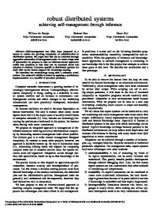
Figure 1: A temperature monitoring sensor network with 54 nodes; the callout shows a dynamic Bayesian network for a subset (t)

of the sensors. Each sensor i observes the temperature Ti

at its location with a fixed additive bias Bi and white Gaussian (t)

noise. The transition model for the temperatures factors as p(T1 Q (t) (t) observation model factors as k p(Zk | Tk , Bk ).

(t−1)

| T1

(t)

) × p(T2

(t−1)

| T1,2

(t)

) × p(T3

(t−1)

| T2,3

) × · · · . The

and network partitions, and we identify and address the belief inconsistency problem that arises in distributed systems.

2

The distributed dynamic inference problem

Following [7], we assume a network model where each node can perform local computations and communicate with other nodes over some channel. The nodes of the network may change over time: existing nodes can fail, and new nodes may be introduced. We assume a message-level error model: messages are either received without error, or they are not received at all. Only the recipient is aware of a successful transmission; neither the sender nor the recipient is aware of a failed transmission. The likelihood of successful transmissions (link qualities) are unknown and can change over time, and link qualities of several node pairs may be correlated. We model the system as a dynamic Bayesian network (dbn). A dbn consists of a set of state processes, X = {X1 , . . . , XL } and a set of observed measurement processes Z = {Z1 , . . . , ZK }; each measurement process Zk corresponds to one of the sensors on one of the nodes. State processes are not associated with unique nodes. A dbn (Figure 1) defines a joint probability model over steps 1 . . . T as1 T T Y Y p(X(t) | X(t−1) ) × p(Z(t) | X(t) ) . p(X(1:T ) , Z(1:T ) ) = p(X(1) ) × | {z } t=2 | {z } t=1 | {z } initial prior

transition model

measurement model

The initial prior is given by a factorized probability model p(X(1) ) ∝ subset of the state processes. The transition model factors as p(X(t) | X(t−1) ) =

L Y

(t)

Q

(1)

h

ψ(Ah ), where each Ah ⊆ X is a

(t)

p(Xi | Pa[Xi ]),

i=1

where

(t) Pa[Xi ]

are the parents of

(t) Xi

in the previous time step. The measurement model factors as

p(Z(t) | X(t) ) =

K Y

(t)

(t)

p(Zk | Pa[Zk ]),

k=1 (t) Pa[Zk ]

(t) Zk

where ⊆ X(t) are the parents of in the current time step. In the distributed dynamic inference problem, each node n is associated with a set of processes Qn ⊆ X; these are the processes about which node n wishes to reason. The nodes need to collaborate so that each (t) node can obtain (an approximation to) the posterior distribution over Qn given all measurements made in (t) (1:t) the network up to the current time step t: p(Qi | z ). We assume that node clocks are synchronized, so that transitions to the next time step are simultaneous. 1 Throughout

this paper, we assume that the DBN has arcs from X(t) to X(t+1) and Z(t) , but nowehere else.

2

X 2, X 3 X 1, X 2, X 3

X 3, X 4

X5 X 3, X 4, X 5

X 2, X 3, X 4

X 5, X 7

X1

X3

X5

X2

X4

X6

X7

X 4, X 5 X 4, X 5, X 6 (a) Junction tree

(b) Markov network

Figure 2: Assumed density filtering for a network of seven temperature sensors. (a) A junction tree for the approximate (t)

(t)

(t)

(t)

(t)

posterior distribution p ˜ , with cliques X1,2,3 , X2,3,4 , X3,4,5 , X4,5,6 , and X5,7 (time indices were omitted for brevity in the (t) Xi

(t) (Ti , Bi )

figure). Each = is a vector consisting of both the temperature and the bias at location i. (b) The corresponding Markov network; dashed edges indicate the edges of the exact distributionin p that are not present in the projection p ˜.

3

Filtering in dynamical systems

The goal of (centralized) filtering is to compute the posterior distribution p(X(t) | z(1:t) ) for t = 1, 2, . . . as the observations z(1) , z(2) , . . . arrive. The basic approach is to recursively compute p(X(t+1) | z(1:t) ) from p(X(t) | z(1:t−1) ) in three steps: 1. Estimation: p(X(t) | z(1:t) ) ∝ p(X(t) | z(1:t−1) ) × p(z(t) | X(t) ); 2. Prediction: p(X(t) , X(t+1) | z(1:t) ) = p(X(t) | z(1:t) ) × p(X(t+1) | X(t) ); R 3. Roll-up: p(X(t+1) | z(1:t) ) = p(x(t) , X(t+1) | z(1:t) ) dx(t) . Thus, in the estimation step we multiply the current belief by the observation likelihood p(z(t) | X(t) ), in the prediction step we multiply in the transition model p(X(t+1) | X(t) ), and finally, in the roll-up step, we marginalize out the state variables X(t) . Exact filtering in dbns is usually expensive or intractable because the belief state rapidly loses all conditional independence structure. An effective approach, proposed by Boyen and Koller [2], hereby denoted “b&k98”, is to periodically project the exact posterior to a distribution that satisfies independence  assertions encoded in a junction tree [3]. Given a junction tree T , with cliques {Ci } and separators Si,j , the projection operation amounts to computing the clique marginals, hence the filtered distribution is approximated as Q (t) ˜ (Ci | z(1:t−1) ) i∈NT p (t) (1:t−1) (t) (1:t−1) p(X | z )≈p ˜ (X | z )= Q , (1) (t) ˜ (Si,j | z(1:t−1) ) {i,j}∈ET p where NT and ET are the nodes and edges of T , respectively. For example, given the junction tree in Figure 2 for a temperature monitoring network with seven nodes, the filtered distribution is approximated as p ˜ (X1 , X2 , X3 ) × p ˜ (X2 , X3 , X4 ) × p ˜ (X3 , X4 , X5 ) × p ˜ (X4 , X5 , X6 ) × p ˜ (X5 , X7 ) p ˜ (X) = . (2) p ˜ (X2 , X3 ) × p ˜ (X3 , X4 ) × p ˜ (X4 , X5 ) × p ˜ (X5 ) (time indices and the conditioning on z(1:t−1) were omitted for brevity). With this representation, the esti(t) (t) mation step is implemented by multiplying each observation likelihood p(zk | Pa[Zk ]) to a clique marginal; the clique and separator potentials are then recomputed with a message passing dynamic programming algorithm, so that the posterior distribution is once again written as a ratio of clique and separator marginals: Q p ˜ (X

(t)

|z

(1:t)

)= Q

(t)

i∈NT

p ˜ (Ci | z(1:t) ) (t)

{i,j}∈ET

p ˜ (Si,j | z(1:t) ) (t+1)

.

The prediction step is performed independently for each clique Ci : we multiply p ˜ (X(t) | z(1:t) ) with the (t+1) (t+1) (t+1) (t+1) transition model p(X | Pa[X ]) for each variable X ∈ Ci and, using variable elimination, (t+1) (1:t) compute the marginals over the clique at the next time step p(Ci |z ).

3

4

Approximate distributed filtering

In principle, the centralized filtering approach described in the previous section could be applied to a distributed system, e.g., by communicating the observations made in the network to a central location that performs all computations, and distributing the answer to every node in the network. While conceptually simple, this approach has substantial drawbacks, including the high communication bandwidth required to scale to a large number of observations, the introduction of a single point of failure to the system, and the fact that nodes do not have valid estimates when the network is partitioned. In this section, we present a distributed filtering algorithm where each node obtains an approximation to the posterior distribution over subset of the state variables. Our estimation step builds on the robust distributed inference algorithm of Paskin et al. [7, 8], while the prediction, roll-up, and projection steps are performed locally at each node.

4.1

Estimation as a robust distributed probabilistic inference

In the distributed inference approach of Paskin et al. [8], the nodes collaborate so that each node n can obtain the posterior distribution over some set of variables Qn given all measurements made throughout the network. In our setting, Qn contains the variables in a subset Ln of the cliques used in our assumed density representation. In their architecture, nodes form a distributed data structure along a routing tree in the network, where each node in this tree is associated with a cluster of variables Dn that includes Qn , as well as any other variables, needed to preserve the flow of information between the nodes, a property equivalent to the running intersection property in junction trees [3]. We refer to this tree as the network junction tree, and, for clarity, we refer to the junction tree used for the assumed density as the external junction tree. Using this architecture, Paskin and Guestrin developed a robust distributed probabilistic inference algorithm, rdpi [7], for static inference settings, where nodes compute the posterior distribution p(Qn | z) over Qn given all measurements throughout the network z. rdpi provides two crucial properties: convergence, if there are no network partitions, these distributed estimates converge to the true posteriors; and, smooth degradation even before convergence, the estimates provide a principled approximation to the true posterior (which introduces additional independence assertions). In rdpi, each node n maintains the current belief βn of p(Qn | z). Initially, node n knows only the marginals of the prior distribution {p(Ci ) : i ∈ Ln } for a subset of cliques Ln in the external junction tree, and its local observation likelihood p(zn | Pa[Zn ]) for each of its sensors. For example, in Figure 3, node 4 initially starts with the prior marginal p(X2 , X3 , X4 ) and the observation likelihood p(z4 | T4 , B4 ) based on its local observation Z4 = z4 . We assume that Pa[Zn ] ⊆ Ci for some clique i ∈ Ln assigned to node n; thus, βn is represented as a collection of priors over cliques of variables, and of observation likelihood functions over these variables. Messages are then sent between neighboring nodes, in an analogous fashion to the sumproduct algorithm for junction trees [3]. However, messages in rdpi are always represented as a collection of priors {πi (Ci )} over cliques of variables Ci , and of measurement likelihood functions {λi (Ci )} over these cliques. This decomposition into prior and likelihood factors is the key to the robustness properties of the algorithm [7]. With sufficient communication, βn converges to p(Qn | z). (t) (t) In our setting, at each time step t, each prior πi (Ci ) is initialized to p(Ci | z(1:t−1) ). The likelihood (t) (t) (t) functions are similarly initialized to λi (Ci ) = p(zi | Ci ), if some sensor makes an observation about (t) these variables, or to 1 otherwise. Through message passing βn converges to p ˜ (Qn | z(1:t) ). An important property of the rdpi algorithm that will be useful in the remainder of the paper is: Property 1. Let βn be the result computed by the rdpi algorithm at convergence at node n. Then the cliques in βn form a subtree of an external junction tree that covers Qn . We will revisit the rdpi algorithm in more detail in Section 5.2.

4.2

Prediction, roll-up and projection

The previous section shows that the estimation step can be implemented in a distributed manner, using (t) rdpi. At convergence, each node n obtains the calibrated marginals p ˜ (Ci | z(1:t) ), for i ∈ Ln . In order to advance to the next time step, each node must perform prediction and roll-up, obtaining the marginals 4

p(z1 | X1) p(X1, X2, X3)

p(z3 | X3) p(X3, X4, X5)

p(z5 | X5) p(X5, X7)

p(z7 | X7) p(X5, X7)

1: X1, X2, X3

3: X2, X3, X4, X5

5: X5, X7

7: X5, X7

2: X2, X3, X4

4: X2, X3, X4, X5

6: X4, X5, X6

p(X2, X3, X4) p(z2 | X2)

p(X2, X3, X4) p(z4 | X4)

p(X4, X5, X6) p(z6 | X6)

Figure 3: Initialization of the rdpi algorithm. Each network node is assigned one or more prior marginals and local observation likelihoods (in this case, exactly one of each). Nodes then build a network junction tree, shown in bold; the underlined variables indicate the variables that were introduced to satisfy the running intersection property. Note that, for each clique Ci in Figure 2, the marginal p(Ci ) is carried by at least one node in the network. Furthermore, the cluster of variables at each node is a superset of the cliques assigned to that node. (t+1)

(t+1)

p ˜ (Ci | z(1:t) ). Recall from Section 3 that, in order to compute a marginal p ˜ (Ci | z(1:t) ), this node (t) (1:t) (t) (1:t) needs p ˜ (X | z ). Due to the conditional independencies encoded in p ˜ (X | z ), it is sufficient to (t+1) obtain a subtree of the external junction tree that covers the parents Pa[Ci ] of all variables in the clique. (t+1) The next time step marginal p ˜ (Ci | z(1:t) ) can then be computed by multiplying this subtree with the (t+1) (t+1) transition model p(X (t+1) | Pa[X (t+1) ]) for each X (t+1) ∈ Ci and eliminating all variables but Ci (t+1) (t) (recall that Pa[X ] ⊆ X ). This procedure suggests the following distributed implementation of prediction, roll-up, and projection: after completing the estimation step, each node selects a subtree of the (global) external junction tree that (t+1) covers Pa[Ci ] and collects the marginals of this tree from other nodes in the network. Unfortunately, this algorithm has substantial drawbacks. First, there may be several subtrees that cover the nodes’ parents and, depending on how the cliques are assigned to nodes in the network, some may be easier to obtain than others. More importantly, it is unclear how to allocate the running time between estimation and collection of marginals in time-critical applications, when the estimation step may not run to completion. Instead, we propose a simple approach that performs both steps at once: run the distributed inference algorithm, described in the previous section, to obtain the posterior distribution over the parents of each clique maintained at the node. This task can be accomplished by including these parent variables in the (t+1) query variables of node n: Pa[Ci ] ⊆ Qn , ∀i ∈ Ln . For example, given the DBN in Figure 1, the query (t) (t) (t) (t) (t+1) (t+1) (t+1) ] = {X1 , X2 , X3 , X4 }. In this manner, , X4 , X3 variables at node 4 need to include Pa[X2 at convergence, the belief β4 at node 4 represents the posterior distribution over (potentially a superset of) (t+1) (t) (t) (t) (t) ˜ (X2,3,4 | z(1:t) ). {X1 , X2 , X3 , X4 }, and the node can compute the marginal p When the estimation step cannot be run to convergence within the allotted time, the variables Scope[βn ] (t+1) covered by the distribution βn that node n obtains may not include the entire parent set Pa[Ci ]. For example, if the nodes are only allowed to communicate once in each time step, node 4 does not receive the prior (t) (t) (t) (t) (t+1) marginal p(X1 , X2 , X3 ), and will thus not have any information about X1 ∈ Pa[X2,3,4 ]. Instead, the (t)

(t)

(t)

(t)

belief β4 will only cover the variables X2 , X3 , X4 (and, potentially, X5 ). In this case, multiplying in the standard transition model is equivalent to assuming a uniform prior for the missing variables, which can lead to very poor solutions in practice. When the transition model is learned from data, p(X (t+1) | Pa[X (t+1) ]) (t+1) (t) (t) is usually computed from the empirical distribution p ˆ (X (t+1) , Pa[X (t+1) ]), e.g., pM LE (X2 | X1 , X 2 ) = (t+1) (t) (t) (t) (t) p ˆ (X2 , X1 , X2 )/ˆ p (X1 , X2 ). Building on these empirical distributions, we can obtain an improved solution for the prediction and roll-up steps, when we do not have a distribution over the entire parent set (t+1) Pa[Ci ]. Specifically, we obtain a valid approximate transition model p ˜ (X (t+1) | W(t) ), where W(t) = Scope[βn ]∩Pa[X (t+1) ], online by simply marginalizing the empirical distribution p ˆ (X (t+1) , Pa[X (t+1) ]) down to p ˆ (X (t+1) , W(t) ). This procedure is equivalent to introducing an additional independence assertion to the model: at time step t + 1, X (t+1) is independent of Pa[X (t+1) ] − W(t) , given W(t) .

5

4.3

Summary of the algorithm

Our distributed approximate filtering algorithm can be summarized as follows: • Using the architecture in [8], construct a network S  junction tree s.t. the query variables Qn at each S (t) (t+1) node n cover C ∪ Pa[C ] . i i i∈Ln i∈Ln • For t = 1, 2, . . ., at each node n, – run rdpi [7] until the end of time step t, obtaining a (possibly approximate) node belief βn ; (t+1) (t) – for each X (t+1) ∈ Ci , i ∈ Ln , compute an approximate transition model p ˜ (X (t+1) | WX ), (t) where WX = Scope[βn ] ∩ Pa[X (t+1) ]; (t+1) (t+1) – for each clique Ci , i ∈ Ln , compute the clique marginal p ˜ (Ci | z(1:t) ) from βn and from (t) (t+1) each p ˜ (X | WX ), locally, using variable elimination. Using the convergence properties of the rdpi algorithm, we prove that, given sufficient communication, our distributed algorithm obtains the same solution as the centralized b&k98 algorithm: Theorem 1. For a set of nodes running our distributed filtering algorithm, if at each time step there is sufficient communication for the rdpi algorithm to converge, and the network is not partitioned, then, for (t) each node n, for each clique i ∈ Ln , the distribution p ˜ (Ci | z(1:t−1) ) obtained by node n is equal to the distribution obtained by running the b&k98 algorithm on the same sequence of observations, with assumed density given by T .

5

Robust distributed filtering

In the previous section, we introduced an algorithm for distributed filtering with dynamic Bayesian networks that, with sufficient communication, converges to the centralized b&k98 algorithm. In some settings, for example when interference causes a network partition, messages may not be propagated long enough to guarantee convergence before nodes must roll-up to the next time step. Consider the example, illustrated in Figure 4, in which a network of cameras localizes itself by observing a moving object. Each camera i carries a clique marginal over the location of the object M (t) , its own camera pose variable C i , and the pose of one of its neighboring cameras: π1 (C 1,2 , M (t) ), π2 (C 2,3 , M (t) ), and π3 (C 3,4 , M (t) ). Suppose communication were interrupted due to a network partition: observations would not propagate, and the marginals carried by the nodes would no longer form a consistent distribution, in the sense that π1 ,π2 ,π3 might not agree on their marginals, e.g., π1 (C 2 , M (t) ) 6= π2 (C 2 , M (t) ). The goal of alignment is to obtain a consistent distribution p ˜ (X(t) | z(1:t−1) ) from marginals π1 , π2 , π3 that is close to the true posterior p(X(t) | z(1:t−1) ) (as measured, for example, by the root-mean-square error of the estimates). For simplicity of notation, we omit time indices t and conditioning on the past evidence z(1:t−1) throughout this section.

5.1

Optimized conditional alignment

One way to define a consistent distribution p ˜ is to start from a root node r, e.g., 1, and allow each clique marginal to decide the conditional density of Ci given its parent, e.g., p ˜1 (C 1:4 , M ) = π1 (C 1,2 , M ) × π2 (C 3 | C 2 , M ) × π3 (C 4 | C 3 , M ). This density p ˜1 forms a coherent distribution over C 1:4 , M , and we say that p ˜1 is rooted at node 1. Thus, π1 fully defines the marginal density over C 1,2 , M , π2 defines the conditional density of C 3 given C 2 , M , and so on. If node 3 were the root, then node 1 would only contribute π1 (C 1 | C 2 , M ), and we would obtain a different approximate distribution. In general, given a collection of marginals πi (Ci ) over the cliques of a junction tree T , and a root node r ∈ NT , the distribution obtained by conditional alignment from r can be written as Y p ˜r (X) = πr (Cr ) × πi (Ci − Sup(i),i | Sup(i),i ), (3) i∈(NT −{r})

where up(i) denotes the upstream neighbor of i on the (unique) path between r and i.

6

1

2

3

4

(a) BK solution

1

2

3

4

1

(b) alignment rooted at 1

2

3

4

(c) alignment rooted at 4

1

2

3

4

(d) min. KL divergence

Figure 4: Alignment results after partition (shown by vertical line). The circles represent 95% confidence intervals in the estimate of the camera location. (a) The exact solution, computed by the BK algorithm in the absence of partitions. (b) Solution obtained when aligning from node 1. (c) Solution obtained when aligning from node 4. (d) Solution obtained by joint optimized alignment.

The choice of the root r often crucially determines how well the aligned distribution p ˜r approximates the true prior. Suppose that, in the example in Figure 4, the nodes on the left side of the partition do not observe the person while the communication is interrupted, and the prior marginals π1 , π2 are uncertain about M . If we were to align the distribution from π2 , multiplying π3 (C 4 | C 3 , M ) into the marginal π2 (C 2,3 , M ) would result in a distribution that is uncertain in both M and C 4 (Figure 4(b)), while a better choice of root could provide a much better estimate (Figure 4(c)). One possible metric to optimize when choosing the root r for the alignment is the entropy of the resulting distribution p ˜r . For example, the entropy of p ˜2 in the previous example can be written as Hp˜2 (C 1:4 , M ) = Hπ2 (C 2,3 , M ) + Hπ3 (C 4 | C 3 , M ) + Hπ1 (C 1 | C 2 , M ),

(4)

where we use the fact that, for Gaussians, the conditional entropy of C 4 given C 3 ,M only depends on the conditional distribution p ˜2 (C 4 | C 3 , M ) = π3 (C 4 | C 3 , M ). A na¨ıve algorithm for obtaining the best root would exploit this decomposition to compute the entropy of each p ˜2 , and pick the root that leads to a lowest total entropy; the running time of this algorithm is O(|NT |2 ). We propose a dynamic programming approach that significantly reduces the running time. Comparing Equation 4 with the entropy of the distribution rooted at a neighboring node 3, we see that they share a common term Hπ1 (C 1 | C 2 , M ), and Hp˜3 (C 1:4 , M ) − Hp˜2 (C 1:4 , M ) = Hπ3 (S2,3 ) − Hπ2 (S2,3 ) , 42,3 . If 42,3 is positive, node 2 is a better root than 3, 42,3 is negative, we have the reverse situation. Thus, when comparing neighboring nodes as root candidates, the difference in entropy of the resulting distribution is simply the difference in entropy their local distributions assign to their separator. This property generalizes to the following dynamic programming algorithm that determines the root r with minimal Hp˜r (X) in O(|NT |) time: • For any node i ∈ NT , define the message from i to its neighbor j as ( 4i,j if mk→i < 0, ∀k 6= j , mi→j = 4i,j + maxk6=j mk→i otherwise where 4i,j = Hπj (Si,j ) − Hπi (Si,j ), and k varies over the neighbors of i in T . • If maxk mk→i < 0 then i is the optimal root; otherwise, up(i) = argmaxk mk→i . Intuitively, the message mi→j represents the loss (entropy) with root node j, compared to the best root on i’s side of the tree: Lemma 1. Let Ti,j denote the subtree rooted at node i, away from node j. Then mi→j is the difference between the entropy of p ˜j and the entropy attained by the best root among the nodes in Ti,j : mi→j = Hp˜j (X) − min Hp˜k (X). k∈Ti,j

7

From Lemma 1, it immediately follows that, if the optimal root is unique, the optimized conditional alignment (oca) algorithm determines the correct root and the upstream neighbors up(i) for each clique i. Ties between root nodes can be resolved locally, by augmenting each entropy message mi→j with the ID of the best root in Ti,j .

5.2

Distributed optimized conditional alignment

In the absence of an additional alignment procedure, rdpi can be viewed as performing conditional alignment. However, the alignment is applied to the local belief at each node, rather than the global distribution, and the nodes may not agree on the choice of the root r. Thus, the network is not guaranteed to reach a globally consistent, aligned distribution. In this section, we show that rdpi can be extended to incorporate the optimized conditional alignment (oca) algorithm from the previous section. By Property 1, at convergence, the priors at each node form a subtree of an external junction tree for the assumed density. Conceptually, if we were to apply oca to this subtree, the node would have an aligned distribution, but nodes may not be consistent with each other. Intuitively, this happens because the optimization messages mi→j were not propagated between different nodes. In rdpi, node n’s belief βn includes a collection of (potentially inconsistent) priors {πi (Ci )}. In the standard sum-product inference algorithm, an inference message µm→n Q from node m to node n is computed by marginalizing out some variables from the factor µ+ , ψ × m→n m k6=n µk→m that combines the messages received from node m’s other neighbors with node m’s local belief. The inference message in rdpi involves a similar marginalization, which corresponds to pruning some cliques from µ+ m→n [6, 7]. When such pruning occurs, any likelihood information λi (Ci ) associated with the pruned clique i is transferred to its neighbor j. Example 1. Consider the example in Figure 5(a) that illustrates the process, in which the rdpi algorithm obtains the posterior distribution over X3 ,X4 ,X5 ,X7 at node 5. When computing an inference message µ4→6 , node 4 combines the incoming messages from its neighbors 2 and 3 with its local belief, by taking a union of the corresponding priors and likelihoods. The resulting factor µ+ 4→6 contains priors and likelihoods over three cliques, {X1 , X2 , X3 }, {X2 , X3 , X4 }, and {X3 , X4 , X5 }. Of these cliques, {X3 , X4 , X5 } is sufficient to compute the conditional distribution over the variables that node 6 reasons about (see Figure 3), given the measurements z1 , . . . , z4 . Specifically, if we were to form the prior distribution over X1 , . . . , X7 using all of the clique marginals held by the nodes in the network (Equation 2) and multiply in the observation likelihoods at each node, we would obtain the posterior distribution p(X1 , . . . , X7 | z1:7 ) ∝

p(X1 , X2 , X3 ) · · · p(X5 , X7 ) × p(z1 | X1 ) × · · · × p(z7 | X7 ) . p(X2 , X3 ) · · · p(X5 ) {z } {z } | | prior marginals

likelihoods

Marginalizing out X1 amounts to removing the clique marginal p(X1 , X2 , X3 ) and passing the observation likelihood p(z1 | X1 ) onto the clique {X2 , X3 , X4 }: X p(x1 , . . . , X7 | z1:7 ) x1

P

x1

∝ |

p(x1 , X2 , X3 )p(z1 | x1 ) p(X2 , X3 , X4 ) · · · p(X5 , X7 ) × × p(z2 | X2 ) × · · · × p(z7 | X7 ) . p(X2 , X3 ) p(X3 , X4 ) · · · p(X5 ) {z } {z } | {z } |

new likelihood λ(X2 , X3 ) = p(z1 | X2 , X3 )

remaining prior marginals

remaining likelihoods

Similarly, marginalizing out X2 amounts to removing the clique marginal p(X2 , X3 , X4 ) and passing the observation likelihood λ(X2 , X3 , X4 ) = p(z1 | X2 , X3 ) × p(z2 | X2 ) × p(z4 | X4 ) onto the clique {X3 , X4 , X5 }. The prior marginal p(X3 , X4 , X5 ), along with the resulting likelihood p(z1,2,3,4 | X3:5 ), form the message from node 4 to node 6. Eventually, node 5 obtains the prior marginals p(X3 , X4 , X5 ),p(X5 , X7 ) and the likelihoods p(z1,2,3,4,6 | X3:5 ),p(z5 | X5 ),p(z7 | X7 ), which are locally combined to form the posterior p(X3 , X4 , X5 , X7 | z1:7 ). In general, if we restrict our attention on messages sent towards a particular node (e.g., 5), whenever a node sends a message to its neighbor, the rdpi algorithm computes one or more new likelihoods λ and 8

p(z7 | X7) p(X5, X7)

p(z1 | X1) p(X1, X2, X3)

1

3

pruned by node 4

5 p(X3, X4, X5) p(z1,2,3,4,6 | X3:5)

p(X1, X2, X3) p(z1 | X1) p(X3, X4, X5) p(z3 | X3)

X 1, X 2, X 3

m123

X 2, X 3, X 4 234

m234

pruned by node 6

2

4 p(X2, X3, X4) p(z2 | X2)

6

X 3, X 4, X 5 345

m456

X 5, X 7 345

X 4, X 5, X 6

p(X3, X4, X5) p(z1,2,3,4 | X3:5)

(a) inference messages

(b) optimization messages

Figure 5: (a) The messages sent towards node 5 at convergence. Each node combines the incoming messages with its local prior marginals and likelihoods (not shown), and prunes redundant cliques not needed by the downstream nodes. For example, in sending a message to its neighbor 5, node 6 combines its local prior and likelihood p(X4 , X5 , X6 ),p(z6 | X6 ) with the incoming message p(X3 , X4 , X5 ),p(z1,2,3,4 | X3:5 ). Since node 5 does not need to reason about the variable X6 , node 6 marginalizes out X6 , thus pruning the clique {X4 , X5 , X6 }. (b) Entropy messages computed in the direction towards node 5. The cliques that were pruned are drawn with dashed line; the remaining cliques {X3 , X4 , X5 } and {X5 , X7 } form the belief β5 at node 5.

removes one or more leaf cliques from external junction tree. Note that while the pruning operation has a global interpretation (removing leaf cliques from the external junction tree), it can be implemented locally, using only the node’s local belief and the incoming messages (e.g., µ2→4 ,µ3→4 ). For the specific procedure that ensures that no clique is ever pruned too early, see [6, 7]. Our distributed oca algorithm piggy-backs on the pruning operation, computing an optimization message mi→j whenever clique i is pruned from clique j (see Figure 5(b)). The optimization message mi→j is stored in clique i; to compute this message, cliques also carry their original, unaligned priors. At convergence, each node will not only have a subtree of an external tree, but also the incoming optimization messages that result from pruning of all other cliques of the external tree. In Figure 5(b), node 5 obtained a subtree X3 X4 X5 —X5 X7 of the external junction tree, and the incoming optimization messages m234→345 ,m456→345 have already been computed (by nodes 4 and 6). Node 5 can now locally compute the remaining optimization messages between the cliques {X3 , X4 , X5 } and {X5 , X7 } and determine if one of its cliques is the root of the conditional alignment. If the optimal root is determined to be {X5 , X7 } then node 5 is the root and, in particular, {X5 , X7 } is the root of the conditional alignment. The alignment, rooted at {X5 , X7 }, is then propagated throughout the network. If the optimal root is {X3 , X4 , X5 } (or another clique upstream) then node 5 aligns itself with respect to clique {X3 , X4 , X5 }. In general, at convergence, each node n is able to determine locally if the optimal root is one of the initial cliques Ln associated with this node or if the alignment ought to be rooted at a different node in the network. Unfortunately, the algorithm, as described so far, does not guarantee that the nodes in the network will make consistent decisions about the optimal root. While the pruned cliques are always leaves of some external junction tree for the assumed density, the external junction trees traced by the pruning operations may differ from one node to another. Continuing Example 1, if we consider the messages sent towards node 1 (Figure 6(a)), we see that the cliques are pruned according to a different junction tree (Figure 6(b)): When node 6 receives the message p(X5 , X7 ),p(z5,7 | X5 , X7 ), it combines this messages with its local belief and prunes the clique {X5 , X7 }, passing the likelihood p(z5,7 | X5 , X7 ) onto the clique {X4 , X5 , X6 }. Hence, {X5 , X7 } is connected to {X4 , X5 , X6 } in 6(b), rather than to {X3 , X4 , X5 }. While the external junction trees in Figures 5(b) and 6(b) are equivalent for inference (in the sense that they have the same cliques and separators), they are not equivalent for the root optimization in oca. For example, if the distribution of X4 given X5 is peaked in the prior marginal π3 (X3 , X4 , X5 ) but not in π6 (X4 , X5 , X6 ), the entropy of the distribution rooted at {X5 , X7 } may be smaller in 5(b) than in 6(b). In order to ensure that the nodes agree on the choice of the external junction tree, we modify the rdpi algorithm as follows. First, we explicitly remove any nondeterminism in the process of forming junction trees in the algorithm. This modification can be implemented simply by defining a lexicographical ordering over the pairs of neighboring clique IDs. In this manner, if two or more pairs of cliques have the same separator, the maximum spanning tree algorithm, used to form the junction tree, connects the pairs with a higher lexicographical order. Second, whenever a network node m sends a message µm→n to its neighbor n in the network junction tree, it includes the clique priors from µn→m in µm→n , omitting any likelihoods and 9

p(z7 | X7) p(X5, X7)

p(z2,3,4,5,6 | X2:4) p(X2, X3, X4)

1

3

p(X5, X7) p(z5,7 | X5,7)

p(X2, X3, X4) p(z2,4 | X2:4) p(X4, X5, X6) p(z5,6 | X4:6)

2

4 p(X2, X3, X4) p(z2 | X2)

pruned by node 3

5 X 1, X 2, X 3

X 2, X 3, X 4

m234

m345

X 4, X 5, X 6

6

pruned by node 6

X 3, X 4, X 5 345

456

m456

X 5, X 7 57

p(X4, X5 , X6) p(z5,6 | X4:6)

(a) messages

(b) pruned cliques

Figure 6: (a) The messages sent towards node 1 at convergence. (b) The external junction tree formed in the order prescribed by the messages in (a). Note that this tree differs from the tree in Figure 6(b).

oca messages. The prior cliques of µn→m are included in µ+ m→n and do not get pruned. By Property 1, given sufficient communication, each node n obtains a subtree of some external junction tree for the assumed density p ˜ . Furthermore, it is easy to see that neighbors in the network junction tree will have overlapping subtrees of the external tree and hence, will have subtrees of a unique external junction tree. Combining these properties, we prove that distributed oca yields a consistent global belief: Theorem 2. Given sufficient communication and in the absence of network partitions, nodes running distributed oca reach a globally consistent belief based on conditional alignment, selecting the root clique that leads to the joint distribution of minimal entropy. In the presence of partitions, each partition will reach a consistent belief that minimizes the entropy within this partition.

5.3

Jointly optimized alignment

While conceptually simple, there are situations where such a rooted alignment will not provide a good aligned distribution. For example, if in the example in Figure 4, cameras 2 and 3 carry marginals π2 (C 2,3 , M ) and π20 (C 2,3 , M ), respectively, and both observe the person, node 2 will have a better estimate of C 2 , while node 3’s estimate of C 3 will be more accurate. If either node is chosen as the root, the aligned distribution will have a worse estimate of the pose of one of the cameras, because performing rooted alignment from either direction effectively overwrites the marginal of the other node. In this example, rather than fixing a root, we want an aligned distribution that attempts to simultaneously optimize the distance to both π2 (C 2,3 , M ) and π20 (C 2,3 , M ). We propose the following optimization problem that minimizes the sum of reverse KL divergence from the aligned distribution to the clique marginals πi (Ci ): X p ˜ (X) = argmin D(q(Ci ) k πi (Ci )), q(X),q|=T

i∈NT

where q |= T denotes the constraint that p ˜ factorizes according to the junction tree T . This method will often provide very good aligned distributions (e.g., Figure (d)). For Gaussian distributions, this optimization problem corresponds to X X minµC ,ΣC − log |ΣCi | + hΣ−1 (µi − µCi )T Σ−1 i , ΣCi i + i (µi − µCi ), i

subject to

i

i∈NT

i∈NT

ΣCi  0,

∀i ∈ NT ,

(5)

where µCi , ΣCi are the means and covariances of q over the variables Ci , and µi , Σi are the means and covariances of the marginals πi . The problem in Equation 5 consists of two independent convex optimization problems over the means and covariances of q, respectively. The former problem can be solved in a distributed manner using distributed linear regression [5], while the latter can be solved using a distributed version of an iterative methods, such as conjugate gradient descent [1]. 10

0.4

0.45 35 nodes 54 nodes

Camera 7

0.4 Camera 10

RMS error

RMS error

0.3

0.2 Camera 3

0.1

0 0

(a) 25-camera testbed

0.35 0.3 0.25

50

100

150 200 time step

250

(b) Convergence, cameras

300

0.2 0

20 40 epochs per time step

60

(c) Convergence, temperature

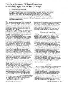
Figure 7: (a) Testbed of 25 cameras used for the SLAT experiments. (b) Convergence results for individual cameras in one experiment. Horizontal lines indicate the corresponding centralized b&k98 solution at the end of the experiment. (c) Convergence versus amount of communication per time step for a temperature network of 54 real sensors.

6

Experimental results

We evaluated our approach on two applications: a camera localization problem [4] (SLAT), in which a set of cameras simultaneously localizes itself by tracking a moving object, and temperature monitoring application, analogous to the one presented in [7]. Figure 7(a) shows some of the 25 ceiling-mounted cameras used to collect the data in our camera experiments. We implemented our distributed algorithm in a network simulator that incorporates message loss and used data from these real sensors as our observations. Figure 7(b) shows the estimates obtained by three cameras in one of our experiments. Note that each camera converges to the estimate obtained by the centralized b&k98 algorithm. In Figure 7(c), we evaluate the sensitivity of the algorithm to incomplete communication on data from the temperature network of 54 real sensors. We see that, with a modest number of rounds of communication performed in each time step, the algorithm obtains a high quality of the solution and converges to the centralized solution. In the second set of experiments, we evaluate the alignment methods, presented in Section 5. In Figure 8(a), the network is split into four components; in each component, the nodes communicate fully, and we evaluate the quality of the solution if the communication were to be restored after a given number of time steps. The vertical axis shows the RMS error of estimated camera locations at the end of the experiment. For the unaligned solution, the nodes may not agree on the estimated pose of a camera, so it is not clear which node’s estimate should be used in the RMS computation; the plot shows an “omniscient envelope” of the RMS error, where, given the (unknown) true camera locations, we select the best and worst estimates available in the network for each camera’s pose. The results show that, in the absence of optimized alignment, inconsistencies can degrade the solution: observations collected after the communication is restored are not sufficient to make up for the errors introduced by the partition. The third experiment evaluates the performance of the distributed algorithm in highly-disconnected scenarios. Here, the sensor network is hierarchically partitioned into smaller disconnected components by selecting a random cut through the largest component. The communication is restored shortly before the end of the experiment. Figures 8(b) shows the importance of aligning from the correct node: the difference between the optimized root and an arbitrarily chosen root is significant, particularly when the network becomes more and more fractured. In our experiments, large errors often resulted from the nodes having uncertain beliefs, hence justifying the objective function. We see that the jointly optimized alignment described in Section 5.3, min. KL, tends to provide the best aligned distribution, though often close to the optimized root, which is simpler to compute. Finally, 8(c) shows the alignment results on the temperature monitoring application. Compared to SLAT, the effects of network partitions on the results for the temperature data are less severe. One contributing factor is that every node in a partition is making local temperature observations, and the approximate transition model for temperatures in each partition is quite accurate, hence all the nodes continue to adjust their estimates meaningfully while the partition is in progress.

11

upper bound

lower bound

0.1

0.8

0.5

fixed root optimized root upper bound min. KL unaligned

upper bound

0.4 RMS error

0.2

1

RMS error

RMS error

0.3

fixed root optimized root unaligned

0.6 0.4

0.3 0.2 lower bound 0.1

0.2 lower bound

0 0

50 100 Duration of the partition

(a) camera localization

0 0

2

4 6 8 Number of partitions

(b) camera localization

10

0 0

fixed root optimized root min. KL unaligned

5 Number of partitions

10

(c) temperature monitoring

Figure 8: Comparison of the alignment methods. (a) RMS error vs. duration of the partition. For the unaligned solution, the plot shows bounds on the RMS error: given the (unknown) true camera locations, we select the best and worst estimates available in the network for each camera’s pose. In the absence of optimized alignment, inconsistencies can degrade the quality of the solution. (b, c) RMS error vs. number of partitions. In camera localization (b), the difference between the optimized alignment and the conditional alignment from an arbitrarily chosen fixed root is significant. For the temperature monitoring (c), the differences are less pronounced, but follow the same trend.

7

Conclusions

This paper presents a new distributed approach to approximate dynamic filtering based on a distributed representation of the assumed density in the network. Distributed filtering is performed by first conditioning on evidence using a robust distributed inference algorithm [7], and then advancing to the next time step locally. With sufficient communication in each time step, our distributed algorithm converges to the centralized b&k98 solution. In addition, we identify a significant challenge for probabilistic inference in dynamical systems: nodes can have inconsistent beliefs about the current state of the system, and an ineffective handling of this situation can lead to very poor estimates of the global state. We address this problem by developing a distributed algorithm that obtains an informative consistent distribution, optimizing over various choices of the root node, and an alternative joint optimization approach that minimizes a KL divergence-based criterion. We demonstrate the effectiveness of our approach on a suite of experimental results on real-world sensor data. Acknowledgments This research was supported by grants NSF-NeTS CNS-0625518 and CNS-0428738 NSF ITR. S. Funiak was supported by the Intel Research Scholar Program; C. Guestrin was partially supported by an Alfred P. Sloan Fellowship.

References [1] D. P. Bertsekas and J. N. Tsitsiklis. Parallel and Distributed Computation: Numerical Methods. Athena Scientific; 1st edition (January 1997), 1997. [2] X. Boyen and D. Koller. Tractable inference for complex stochastic processes. In Proc. of UAI, 1998. [3] R. Cowell, P. Dawid, S. Lauritzen, and D. Spiegelhalter. Probabilistic Networks and Expert Systems. Springer, New York, NY, 1999. [4] S. Funiak, C. Guestrin, M. Paskin, and R. Sukthankar. Distributed localization of networked cameras. In Proc. of Fifth International Conference on Information Processing in Sensor Networks (IPSN-06), 2006. [5] C. Guestrin, R. Thibaux, P. Bodik, M. A. Paskin, and S. Madden. Distributed regression: an efficient framework for modeling sensor network data. In Proc. of IPSN, 2004. [6] M. Paskin. Exploiting Locality in Probabilistic Inference. PhD thesis, University of California, Berkeley, September 2004. [7] M. A. Paskin and C. E. Guestrin. Robust probabilistic inference in distributed systems. In UAI, 2004. [8] M. A. Paskin, C. E. Guestrin, and J. McFadden. A robust architecture for inference in sensor networks. In Proc. of IPSN, 2005. [9] A. Pfeffer and T. Tai. Asynchronous dynamic Bayesian networks. In Proc. UAI 2005, 2005. [10] M. Rosencrantz, G. Gordon, and S. Thrun. Decentralized sensor fusion with distributed particle filters. In Proc. of UAI, 2003. [11] F. Zhao, J. Liu, J. Liu, L. Guibas, and J. Reich. Collaborative signal and information processing: An information directed approach. Proceedings of the IEEE, 91(8):1199–1209, 2003.

12

Carnegie Mellon University 5000 Forbes Avenue Pittsburgh, PA 15213

Carnegie Mellon University does not discriminate and Carnegie Mellon University is required not to discriminate in admission, employment, or administration of its programs or activities on the basis of race, color, national origin, sex or handicap in violation of Title VI of the Civil Rights Act of 1964, Title IX of the Educational Amendments of 1972 and Section 504 of the Rehabilitation Act of 1973 or other federal, state, or local laws or executive orders. In addition, Carnegie Mellon University does not discriminate in admission, employment or administration of its programs on the basis of religion, creed, ancestry, belief, age, veteran status, sexual orientation or in violation of federal, state, or local laws or executive orders. However, in the judgment of the Carnegie Mellon Human Relations Commission, the Department of Defense policy of, "Don't ask, don't tell, don't pursue," excludes openly gay, lesbian and bisexual students from receiving ROTC scholarships or serving in the military. Nevertheless, all ROTC classes at Carnegie Mellon University are available to all students. Inquiries concerning application of these statements should be directed to the Provost, Carnegie Mellon University, 5000 Forbes Avenue, Pittsburgh PA 15213, telephone (412) 268-6684 or the Vice President for Enrollment, Carnegie Mellon University, 5000 Forbes Avenue, Pittsburgh PA 15213, telephone (412) 268-2056 Obtain general information about Carnegie Mellon University by calling (412) 268-2000