Myers (1982) for the case of one categorical variable. One then .... giving them small weights, whereas vertical outliers have only a small e ect on the L1 stage. However ... algorithm proposed by Rousseeuw and Leroy (1987, page 259-260). The L1 ..... P. Bickel, K. Doksum, and J.L. Hodges, Jr., Belmont: Wadsworth. Draper ...
Robust regression with both continuous and binary regressors Mia Hubert and Peter J. Rousseeuw
Department of Mathematics and Computer Science, U.I.A., Universiteitsplein 1, B-2610 Antwerp, Belgium Abstract: We present a robust regression method for situations where there are continuous as well as binary regressors. The latter are often the result of encoding one or more categorical variables. In the rst step we downweight leverage points by computing robust distances in the space of the continuous regressors. Then we perform a weighted least absolute values t in function of the continuous as well as the binary regressors. Finally, the error scale is estimated robustly. We pay particular attention to the two-way model, in which the proposed estimator is compared with an algorithm that treats the continuous and the categorical variables alternatingly. An S-PLUS function for the proposed estimator is given, and used to analyze a recent data set from economics. Keywords: Analysis of Covariance; Median Polish; Minimum Volume Ellipsoid Estimator; Outlier Detection; Robust Distance; Weighted Least Absolute Values. AMS Subject Classi cation: 62F35, 62J05 Brief running title: CONTINUOUS AND BINARY REGRESSORS
1 Introduction In the classical linear regression model
yi = � 0 +
p X j =1
where ei � N (0; �2); i = 1; : : : ; n
�j xij + ei
(1.1)
the explanatory variables xij are often quantitative. We now consider a model in which also qualitative variables are included. This situation often occurs in the social and economical sciences, where the explanatory variables may include gender, ethnic background, professional occupation, marital status and so on. The usual convention is to encode such categorical regressors by binary dummy variables. If we have m categorical variables with c1; : : : ; cm levels, we can write
yi = � 0 +
p X j =1
�j xij +
q X l=1
lIil + ei
(1.2)
where each Iil is either 0 or 1, and where q = Pmk=1(ck ? 1) since coding a categorical variable with c levels is done with c ? 1 dummy variables. Actually, (1.2) is more general because the binary variables do not have to be the result of encoding categorical variables, hence other situations with dummy variables are covered also. To x ideas, let us consider a situation with two categorical variables (m = 2) as is often encountered in practice. Model (1.2) can then be written as
yi = �0 +
p X j =1
�j xij +
cX 1 ?1 k=1
�k Iik +
cX 2 ?1 l=1
l Jil + ei :
(1.3)
The observations thus correspond to cell entries in a two-way table with c1 rows and c2 columns. The slope parameters are constant over all cells, but the intercept is not. For an arbitrary value of m we obtain an m?way table. We will allow the number of observations to vary between cells. Also empty cells may occur, although an entirely empty cross-section is not permitted. (A cross-section consists of all the observations belonging to a xed level of any categorical variable.) In the latter case the empty level should be removed, since its coe�cient is not estimable from the data. In general, our aim is to construct a robust estimator of the parameters �j and l in (1.2). The least squares method (LS ) ts the model (1.2) in a nonrobust way, by applying the standard calculations with p + q regressors. It treats the dummies in the same way as 1
the continuous regressors (see, e.g., Draper and Smith (1981) and Hardy (1993)). However, it is well-known that the LS method is very sensitive to outliers. The least absolute values (L1 ) method as implemented by Armstrong and Frome (1977) is robust against outliers in the y?direction, but does not protect against points of which (xi1 ; : : : ; xip) is outlying. Such observations will be called leverage points. A frequently used method of robust regression is M ?estimation (also LS and L1 belong to this class). This approach can also be applied to the model (1.2), as done by Birch and Myers (1982) for the case of one categorical variable. One then has to solve a system of p + q +1 implicit equations, e.g. using an iteratively reweighted least squares algorithm. But M -estimators are still vulnerable to leverage points. Therefore it seems natural to try to extend regression methods that can withstand a positive percentage of contamination, including leverage points. Typical examples are the least median of squares (LMS) estimator and the least trimmed squares (LTS) estimator (Rousseeuw 1984), and the class of S-estimators (Rousseeuw and Yohai 1984). However, we cannot simply run these estimators on (1.2) by treating the dummy variables in the same way as the continuous regressors, since this would lead to a problem of singular matrices. The typical algorithm for LMS regression in the model (1.1) starts by drawing a subset of p + 1 observations. Then the hyperplane through these p + 1 points is obtained, and the corresponding objective function computed. This procedure is repeated often, and the best t is kept. But in the case of p + q regressors of which q are binary variables, the large majority of (p + q + 1)?subsets will be of less than full rank, hence the hyperplanes cannot be computed. The algorithm of Stromberg (1993) faces the same problem. In the next section we will describe the proposed estimator. Section 3 studies the special case when there are two categorical variables in the model. A real example is worked out in Section 4. Finally, the Appendix provides S-PLUS code for the proposed algorithm.
2 Description of the estimator RDL1 In this section we describe a new method for the general model (1.2). It consists of three stages. In the rst stage we identify leverage points, and in the second stage these are downweighted when estimating the parameters. The nal step estimates the residual scale. In the rst stage we look for leverage points, i.e. outliers in the set X = 2
fx1 ; : : : ; xi; : : : ; xng where the components of xi = (xi1; : : : ; xip) are the continuous regres-
sors. Therefore X is a data set in p dimensions. To these data we apply the minimum volume ellipsoid estimator (MVE) introduced in (Rousseeuw 1985). It consists of a robust location estimator T (X ) de ned as the center of the smallest ellipsoid containing half of X , as well as a scatter matrix C (X ) given by the shape of that ellipsoid. One can then compute the robust distances de ned as q
RD(xi) = (xi ? T (X ))C (X )?1(xi ? T (X ))t
(2.1)
(Rousseeuw and Leroy 1987, pp. 265-269). If the xi are observational (rather than designed) with a multivariate gaussian distribution, T (X ) and C (X ) are consistent for the underlying parameters (Davies 1992). For large n the (RD(xi))2 would thus be roughly �2p distributed. Consequently, observations for which RD(xi) is unusually large relative to that distribution can be identi ed as leverage points. Based on the robust distances RD(xi), we compute strictly positive weights wi by wi = minf1; RDp(x )2 g (2.2) i for i = 1; : : : ; n. (The numerator p in (2.2) is the expected value of the chi-square distribution �2p mentioned above.) By using strictly positive weights wi no observations are entirely left out, thus no extra empty cells are created. In the second step, the parameters (�; ) of the model (1.2) are estimated by a weighted L1 procedure n X minimize wijri(�; )j (2.3) �;
i=1
applied to the observations (yi; 1; xi1; : : : ; xip; Ii1; : : : ; Iiq ). The solution (�^ ; ^ ) can e.g. be found using the least absolute values algorithm of Barrodale and Roberts (1973), who do not make a distinction between the continuous and discrete variables. Armstrong and Frome (1977) developed a faster L1 algorithm which treats the two types of variables separately. In the third and last step, the scale of the residuals is estimated by
�^ = 1:4826 median jrij i
(2.4)
where the constant 1.4826 makes the estimator consistent at gaussian errors. The entire three-stage procedure using (2.1) to (2.4) will be called the RDL1 estimator because it uses Robust Distances and L1 regression. The robust estimate (�^ ; ^ ; �^ ) can now 3
be used to detect regression outliers, by agging the observations whose absolute standardized residual jri=�^ j exceeds 2.5. The nite-sample e�ciency of the estimators can then be increased by applying reweighted least squares to the data set, with weights depending on jri=�^ j. This also makes approximate inference available. The nite-sample breakdown value "�n of an estimator (Donoho and Huber, 1983) measures the maximum percentage of observations that can be replaced while leaving the estimate bounded. By construction, the estimator RDL1 protects against leverage points by giving them small weights, whereas vertical outliers have only a small e�ect on the L1 stage. However, an exact formula of the breakdown value of the RDL1 procedure seems hard to nd. At any rate, if the binary variables form an m?way table where each cell contains exactly one observation, we have the upper bound 2
1 m n� Y
"�
j =1
cj
mY ?1
61 + 6 j =1 6 6 6 2 4
3
c(j) 77 7 7 7 5
� 2c1
(2.5)
(m)
on the breakdown value of any regression equivariant estimator. Here, c(j) denotes the j-th smallest level among the m categorical variables. The upper bound (2.5) can be explained as follows. In the model (1.2), denote by r the rank of the set of binary vectors fIi = (Ii1 ; : : : ; Iiq ); 1 � i � ng. Then the breakdown value of any regression equivariant estimator of (�0; 1; : : : ; q ) is bounded above by (see, e.g., Mili and Coakley 1996) 1 �n ? N + 1� ; (2.6) n 2 where n denotes the number of observations and N is the maximum number of points Ii which lie in an (r ? 1) dimensional plane. Here, the points Ii determine an m-way table with c1 : : : cm levels. Since the complement of any cross-section of this table determines a hyperplane, N equals
n ? minimum number of observations in a cross-section: m Y
m Y
mY ?1
If all cells contain one observation, we have n = cj and N = cj ? c(j). Inserting j =1 j =1 j =1 these expressions in (2.6) leads directly to the upper bound (2.5).
4
Computational aspects Our estimator RDL1 can easily be implemented in S-PLUS (1993), because both the MVE and the L1 estimator are built-in functions. The MVE estimates are obtained from the function cov.mve which uses a genetic algorithm. A special case of this algorithm, obtained by setting popsize=1, births.n=0 and maxslen=p +1, corresponds to the original resampling algorithm proposed by Rousseeuw and Leroy (1987, page 259-260). The L1 computation in the S-PLUS function l1 t is based on the algorithm of Barrodale and Roberts (1973). Note that the weighted least absolute values problem on a data set (xi; yi) can be reduced to the least absolute values problem on the set (~xi; y~i) obtained by the transformation x~ i = wi xi
and
y~i = wiyi:
The S-PLUS code of the whole RDL1 procedure is given in the appendix. Alternatively, one can make use of the Fortran library ROBETH (Marazzi 1993), which also includes procedures for the MVE and L1 estimators.
3 The two-way layout In this section we will focus on the case of two categorical variables (m = 2). For this we shall use the notation of (1.3). In many two-way applications there is only a single observation per cell. This observation is often already a summary of actual data values, which are not available to the statistician. We then have to estimate p + c1 + c2 ? 1 parameters from only c1c2 data points. This is quite di�erent from the one-way layout (m = 1), which assumes several observations for each level of the categorical variable. In that case we can estimate the parameters by least median of squares regression using a modi ed resampling algorithm, as described in Hubert and Rousseeuw (1996). We already pointed out in Section 1 why such an algorithm does not work well for more than one categorical variable. For the two-way layout we also developed an alternative estimator, denoted as POL1. The POL1 method is also a new proposal, but we do not recommend it because its convergence is not guaranteed. Therefore, we will only use it to compare the RDL1 method with. The POL1 algorithm is de ned by an iterative procedure which makes use of the twoway structure of the intercepts. In fact, the response yi is on the one hand explained by 5
the quantitative variables, and on the other hand by two qualitative variables. The former dependence can be analyzed by means of a linear model, and the latter by means of a two-way table. The POL1 method carries out both steps alternatingly. The skeleton of the POL1 algorithm is as follows: 1. Initialize the residuals as ri
yi .
2. Using only the continuous regressors, apply a robust regression estimator on the (xi; ri), yielding (�^0 ; �^1 ; : : : ; �^p). Put ri ri ? �^0 ? Pj �^j xij . 3. Using only the categorical variables, apply a robust technique for estimating the e�ects in a two-way table, here formed by the residuals obtained in step 2. Having the estimated e�ects (�^0 ; �^1; : : : ; �^c1?1; ^1; : : : ; ^c2?1), form new residuals ri ri ? �^0 ? P ^k Iik ? Pl ^l Jil . k� 4. Repeat steps 2 and 3 until convergence. The nal estimates (�^0 ; �^1 ; : : : ; �^p; �^1 ; : : : ; �^c1?1 ; ^1; : : : ; ^c2?1) are taken as the sum of the estimates calculated in the iterations. We did not yet specify the robust estimators in steps 2 and 3. For the two-way table in step 3 we can use the median polish procedure of Tukey (1977). This is an iterative method where the estimates are obtained by subtracting row medians from the current cell entries, then subtracting column medians, and so on. This process is repeated until all rows and columns have zero median. In practice, a few iterations are usually su�cient. The median polish method can be seen as an approximation to the least absolute values estimate for a two-way table. A detailed account was given by Hoaglin, Mosteller and Tukey (1983). The median polish method is easy to implement, and is incorporated in S-PLUS. In step 2 of the POL1 algorithm we carry out an L1 regression on the observations whose q robust distances RD(xi) do not exceed �2p;0:975 . This is a fast robust method, described in Rousseeuw and Van Zomeren (1992). Note that the RD(xi) need not be calculated at each POL1 iteration step, as the explanatory variables xi remain the same. The median polish q in step 3 is applied to the same observations with RD(xi) � �2p;0:975. The abbreviation POL1 of the overall method stems from the combination of median POlish and L1 . The POL1 iterations are stopped if the norm of the new slope estimate �^ in step 2 is less than a given precision, which in our program was set to 10?5. We carried out several 6
Table 1: Real data set with four continuous and two categorical regressors region 1 2 3 4 5 6 7 8 9 10 11 12 13 14 15 16 17 18 19 20 21
PA 46.84 35.54 28.42 32.54 28.92 36.61 34.71 24.32 35.15 34.06 37.94 35.88 31.28 33.61 33.86 43.24 42.65 37.19 49.70 41.96 28.86
GPA -2.60 -1.42 -1.48 -4.51 -0.88 -1.39 -2.22 -5.11 -0.16 -3.86 -4.61 -2.17 -1.90 2.02 0.75 -4.41 -2.28 -2.75 -4.86 -4.59 -2.11
period 1 period 2 HS GHS y PA GPA HS 1.68 0.20 0.97 44.24 3.80 1.88 1.67 0.63 2.14 34.12 -3.33 2.30 1.71 0.12 6.13 26.94 -1.71 1.83 1.37 0.32 7.36 28.03 -0.89 1.69 2.14 -0.08 3.63 28.04 -1.47 2.06 3.00 0.45 -4.30 35.22 -2.87 3.45 2.94 0.27 2.06 32.49 -1.89 3.21 3.57 -0.55 -18.64 19.21 0.36 3.02 3.27 0.03 5.15 34.99 -4.95 3.30 2.74 0.19 6.88 30.20 -3.02 2.93 2.07 0.38 -1.24 33.33 0.06 2.45 1.57 -0.11 -1.31 33.71 -4.67 1.46 2.74 -0.57 1.73 29.38 -2.74 2.17 1.92 0.32 0.44 35.63 -0.51 2.24 0.86 0.46 -15.53 34.61 -5.36 1.32 1.82 0.52 -10.99 38.83 -6.83 2.34 1.52 -0.17 0.60 40.37 -3.94 1.35 2.39 0.40 3.71 34.44 1.37 2.79 1.16 0.09 -2.38 44.84 -7.70 1.25 2.00 -0.12 -1.35 37.37 -5.87 1.88 5.17 0.46 -1.08 26.75 -1.83 5.63
GHS 0.13 1.04 1.28 0.35 -0.81 0.59 1.88 2.98 0.68 0.48 0.24 2.59 0.07 0.62 0.61 0.71 0.45 1.27 0.80 0.80 1.35
y 8.47 2.76 24.08 13.97 0.63 -1.99 13.10 15.42 19.65 8.45 9.04 9.47 24.18 9.09 -1.89 14.62 -0.44 17.84 10.95 -1.55 -1.66
PA 48.04 30.79 25.23 27.14 26.57 32.35 30.60 19.57 30.04 27.18 33.39 29.04 26.64 35.12 29.25 32.00 36.43 35.81 37.14 31.50 24.92
GPA -4.03 -3.10 -4.29 -2.45 1.31 -1.25 -3.21 2.48 -0.79 -1.14 -0.42 1.40 1.04 -0.81 -2.56 1.68 1.00 -2.29 1.59 0.70 -0.14
period 3 HS 2.01 3.34 3.11 2.04 1.25 4.04 5.09 6.00 3.98 3.41 2.69 4.05 2.24 2.86 1.93 3.05 1.80 4.06 2.05 2.68 6.98
GHS 0.40 0.25 0.88 1.95 0.67 0.23 -0.17 2.27 0.55 0.28 -0.18 -0.05 0.12 0.25 0.30 0.78 0.37 0.18 0.82 -0.17 0.59
y 3.72 9.29 25.59 27.41 18.32 11.20 21.95 33.03 22.02 13.68 11.24 15.06 10.73 1.53 11.37 -0.07 14.17 8.05 15.96 9.91 6.94
simulations (with one observation per cell) to investigate the algorithm. It converged in most cases, but sometimes diverged. Therefore, we do not recommend the POL1 method in practice. We will compare it with the RDL1 in the example below.
4 Example To illustrate the RDL1 method we consider an economics data set (Table 1) from Wagner (1994). He investigates the rate of employment growth (variable y) as a function of the percentage of people engaged in production activities (variable PA) and higher services (variable HS), and of the growth of these percentages (variables GPA and GHS). The response also depends on the geographical region and the time period. The data set considers 21 regions around Hannover, and three time periods: 1979-1982, 1983-1988, and 1989-1992. The model thus contains 4 continuous and 2 categorical regressors. For each cell there is only one data point available, so the total number of observations equals 63. 7
Table 2: Weights and standardized residuals region 1 2 3 4 5 6 7 8 9 10 11 12 13 14 15 16 17 18 19 20 21
wi .70 1.0 1.0 .91 1.0 1.0 1.0 .21 1.0 1.0 1.0 1.0 .50 .93 .78 1.0 .82 1.0 .49 .92 .47
period 1 LS POL1 RDL1 .18 .13 0.0 .83 .32 3.5 -.38 -1.4 0.0 .12 .07 0.0 -.32 -.97 0.0 .03 0.0 0.0 .01 -1.5 0.0 -1.2 0.0 -.51 -2.1 0.0 .65 1.1 2.9 -.45 -.81 -1.9 .79 -.09 0.0 -.90 0.0 0.0 .29 0.0 0.0 -1.2 -4.3 -1.3 -.48 0.0 0.0 .42 0.0 0.0 .39 .71 0.0 -.07 -.07 .94 .68 .77 1.9 1.2 .64 0.0
wi .23 1.0 .43 1.0 .25 1.0 .18 .06 1.0 1.0 1.0 .10 1.0 1.0 .93 .83 1.0 .29 .50 1.0 .18
period 2 LS POL1 RDL1 .41 0.0 2.7 -.69 -.62 0.0 .54 2.0 3.2 -.08 -.07 0.0 -.69 -1.8 -2.3 -.80 -.20 -2.2 -.80 -.75 -.21 .18 7.3 .57 1.9 1.4 -.43 0.0 -.04 .04 0.0 0.0 -.79 .53 -2.4 1.8 5.7 5.4 .66 2.1 1.5 -.06 0.0 0.0 2.1 6.4 4.4 -.97 -1.2 -4.2 .61 2.1 3.0 .38 2.7 0.0 -1.1 -.78 -3.4 -.93 -1.5 -3.8
8
wi .63 1.0 .53 .18 .56 1.0 .41 .07 1.0 1.0 1.0 .80 1.0 1.0 1.0 .62 1.0 1.0 .49 1.0 .16
period 3 LS POL1 RDL1 -.59 -.63 -1.6 -.14 0.0 0.0 -.16 1.4 .41 -.04 1.6 .90 1.0 1.0 2.6 .77 2.0 .90 .79 1.5 1.7 1.1 - 13.0 -.06 0.0 0.0 -.22 -.22 0.0 .41 .01 0.0 0.0 0.1 0.0 -.90 -.28 -.67 -.94 -1.1 -2.7 1.3 1.7 2.2 -1.6 -1.7 -2.8 .55 .47 .01 -1.0 -.71 -2.0 -.31 0.0 0.0 .39 0.0 0.0 -.25 -.64 -1.9
Table 2 lists the weights wi de ned by (2.2), and the standardized residuals obtained by the LS; POL 1 and RDL1 estimators. The residuals were divided by the classical scale q estimate �^ = (n ? p ? q ? 1)?1 Pn1 ri2 for LS , and by (2.4) for the robust methods. The least squares residuals do not reveal any outlier. This is also seen in Figure 1 which plots the standardized residuals ri =�^, none of which exceeds 2.5 in absolute value. On the other hand, both robust methods indicate the presence of outliers. The large residuals are boldfaced in Table 2, and lie outside their tolerance band in Figure 1. The RDL1 method detects several outliers, whereas the iterative algorithm POL1 nds only three (we do not consider residuals near the tolerance band to be outliers). A disadvantage of the POL1 method is that it can create empty cross-sections, so that certain estimates and residuals are unde ned. Here, this happens for region 8 (Laatzen). This problem cannot occur with the RDL1 method. Note that the most extreme residuals obtained by RDL1 correspond with the same region 8, in time periods 2 and 3. In Figure 1, we see that the residual plot of RDL1 is more informative than that of POL1, which is still quite similar in shape to the classical LS plot. Based on the properties of both robust methods, as illustrated in this example, we strongly recommend the RDL1 method in practice. It is easier to implement than POL1, runs faster, always converges, does not create empty cells, and in our experience yields more robust results. A minor artefact of the RDL1 plot in Figure 1 are the zero residuals produced by the L1 t. If one wants to remove this e�ect, a simple and e�ective way is to append a fourth step to the RDL1 algorithm. This nal step computes a reweighted least squares (RLS) t, in which the weight vi of each observation depends on its RDL1 residual jri=�^j. For the example, the RLS t is shown in the lower portion of Figure 1. In general, computing an RLS t starting from a robust initial estimate tends to increase the nite-sample e�ciency (see the simulations in Rousseeuw and Leroy 1987, pp. 208-214). Moreover, the RLS yields the usual inferential output such as t-statistics and F-statistics. Note that the corresponding p-values are approximative, since they assume that the weights vi have correctly identi ed the cases generated by the model (1.2).
9
10
period 1
period 2
period 3
0
5
LS • •• •• • • •• • •• •• • • • • •• • • • • •• • •• • • • • • •• •• •• • • •• •• • •• •• • • • •• • • • •• •• • • •• •• • • •• •• •• • • •• • • • • • •
10
1
11
21 1
11
21 1
POL1
• • • •• • • • • • •• • • • • •• •• •• •• •• • •• •• • •• •• •• •• •• •• •• • • •• • • • • • • •• • • •• • • •• •• • • • • • • • • • • •• • • • • • 1
11
21 1
11
21 1
11
10
•
0
5
RDL1 •
•8 •
• •••••••
•
1
11
• • • •• • • •
••
•• • • • •
•• ••
•
• •• • •
21 1
11
••
•
•
• •
• ••
•• •
10 5
RLS
21
8
•• •• • ••• • ••••• • •• • • • • •
21 1
11
• •8
21
8
• • • • • • • • • • • •• • • • • • • • • •• • • •• • • • • • • • • • • • • • • •• • • • • •• • •• • • • • • • • • •• •• • • • •• •• •• ••
0
21
•
•
5 0
11
1
••
11
21 1
11
21 1
11
21
Figure 1: Index plots of the standardized residuals produced by least squares (LS ), the POL1 method, the RDL1 method, and reweighted least squares (RLS ) based on the RDL1 results. 10
5 Appendix Below is an S-PLUS implementation of the proposed estimator RDL1 . It is very short because both the MVE estimator and L1 tting are intrinsic in S-PLUS. (Note that the current version of the function cov.mve cannot handle the univariate case p = 1, hence the code below computes the sample median and the mad in that case, yielding the robust distance RD(xi ) = (xi ? medianj xj )=(madj xj ) instead.) rdl1.s