Robust Semidefinite Programming - ISyE

Robust Semidefinite Programming∗ Aharon Ben-Tal†

Laurent El Ghaoui‡

Arkadi Nemirovski§

August 1st, 1998

Abstract In this paper, we consider semidefinite programs where the data is only known to belong to some uncertainty set U. Following recent work by the authors, we develop the notion of robust solution to such problems, which are required to satisfy the (uncertain) constraints whatever the value of the data in U. Even when the decision variable is fixed, checking robust feasibility is in general NP-hard. For a number of uncertainty sets U, we show how to compute robust solutions, based on a sufficient condition for robust feasibility, via SDP. We detail some cases when the sufficient condition is also necessary, such as linear programming or convex quadratic programming with ellipsoidal uncertainty. Finally, we provide examples, taken from interval computations and truss topology design.

1

Introduction

1.1

SDPs with uncertain data

We consider a semidefinite programming problem (SDP) of the form max bT y subject to F (y) = F0 +

m X

yi Fi º 0,

(1)

i=1

where b ∈ Rm is given, and F is an affine map from y ∈ Rm to S n . In many practical applications, the “data” of the problem (the vector b and the coefficients matrices F0 , . . . , Fm ) is subject to possibly large uncertainties. Reasons for this include the following. • Uncertainty about the future. The exact value of the data is unknown at the time the values of y should be determined and will be known only in the future. (In a risk management problem for example, the data may depend on future demands, market prices, etc, that are unknown when the decision has to be taken.) ∗ This research was partly supported by the Fund for the Promotion of Research at the Technion, by the G.I.F. contract No. I-0455-214.06/95, by the Israel Ministry of Science grant # 9636-1-96, and by Electricit´e de France, under contract P33L74/2M7570/EP777. † Faculty of Industrial Engineering and Management, Technion – The Israel Institute of Technology, Technion City, Haifa 32000, Israel; e-mail: [email protected] ‡ Ecole Nationale Suprieure de Techniques Avances, 32, Bvd. Victor, 75739 Paris, France; email: [email protected]. § Faculty of Industrial Engineering and Management, Technion - The Israel Institute of Technology, Technion City, Haifa 32000, Israel; e-mail: [email protected]

1

• Errors in the data. The data originates from a process (measurements, computational process) that is very hard to perform error-free (errors in the measurement of material properties in a truss optimization problem, sensor errors in a control system, floating-point errors made during computation, etc). • Implementation errors. The computed optimal solution y ∗ cannot be implemented exactly, which results in uncertainty about the feasibility of the implemented solution. For example, the coefficients of an optimal finite-impulse response (FIR) filter can often be implemented in 8 bits only. As it turns out, this can be modeled as uncertainties in the coefficients matrices Fi . • Approximating nonlinearity by uncertainty. The mapping F (y) is completely known, but (slightly) non linear. The optimizer chooses to approximate the nonlinearity by uncertainty in the data. • Infinite number of constraints. The problem is posed with an infinite number of constraints, indexed on a scalar parameter ω (for example, the constraints express a property of a FIR filter at each frequency ω). It may be convenient to view this parameter as a perturbation, and regard the semi-infinite problem as a robustness problem. Depending on the assumptions on the nature of uncertainty, several methods have been proposed in the Operations Research/Engineering literature. Stochastic programming works with random perturbations and probabilities of satisfaction of constraints, and thus requires correct estimates of the distribution of uncertainties; sensitivity analysis assumes the perturbations is infinitesimal, and can be used only as a “post-optimization” tool; the “Robust Mathematical Programming” approach recently proposed by Mulvey, Vanderbei and Zenios [13] is based on the (sometimes very restrictive) assumption that the uncertainty takes a finite number of values (corresponding to “worst-case scenarios”). Interval arithmetic is one of the methods that have been proposed to deal with uncertainty in numerical computations; references to this large field of study include the book by one of its founders, Moore [12], the more recent book by Hansen [9], and also the very extensive web site developed by Kosheler and Kreinovich [11]. The approach proposed here assumes (following the philosophy of interval calculus) that the data of the problem is only known to belong to some “uncertainty set” U; in this sense, the perturbation to the nominal problem is deterministic, unknown-but-bounded. A robust solution of the problem is one which satisfies the perturbed constraints for every value of the data within the admissible region U. The robust counterpart of the SDP is to minimize the worst-case value of the objective, among all robust solutions. This approach was introduced by the authors independently in [1, 2, 3] and [15, 5]; although apparently new in mathematical programming, the notion of robustness is quite classical in control theory (and practice). Even for simple uncertainty sets U, the resulting robust SDP is NP-hard. Our main result is to show how to compute, via SDP, upper bounds for the robust counterpart. Contrarily to the other approaches to uncertainty, the robust method provides (in polynomial time) guarantees (of,e.g., feasibility), at the expense of possible conservatism. Note that there is no real conflict between other approaches to uncertainty and ours; for example, it is possible to solve via robust SDP a stochastic programming problem with unknown-but-bounded distribution of the random parameters.

1.2

Problem definition

To make our problem mathematically precise, we assume that the perturbed constraint is of the form F(y, δ) º 0, 2

where y ∈ Rm is the decision vector, δ is a “perturbation vector” that is only known to belong to some “perturbation set” D ⊆ Rl , and F is a mapping from Rm × D to S n . We assume that F(y, δ) is affine in y for each δ, and rational in δ for each y; also we assume that D contains 0, and that F(y, 0) = F (y) for every y. Without loss of generality, we assume that the objective vector b is independent of perturbation. We consider the following problem, referred to as the robust counterpart to the “nominal” problem (1): max bT y subject to y ∈ XD (2) where XD is the set of robust feasible solutions, that is, n

¯ ¯

XD = y ∈ Rm ¯ for every δ ∈ D, F(y, δ) is well-defined and F(y, δ) º 0

o

.

In this paper, we only consider ellipsoidal uncertainty. This means that the perturbation set D consists of block vectors, each block being subject to an Euclidean-norm bound. Precisely,   

 ¯  1  ¯ δ   ¯   ¯ D = δ ∈ Rl ¯ δ =  ...  , where δ k ∈ Rnk , kδ k k2 ≤ ρ, k = 1, . . . , N ,  ¯    ¯ δN

(3)

where ρ ≥ 0 is a given parameter that determines the “size” of the uncertainty, and the integers nk denote the lengths of each block vector δk (we have of course n1 + . . . + nN = L). There are many motivations for considering the above framework. It can be used when the perturbation is a vector with each component bounded in magnitude, in which case each block vector δ k is actually a scalar (n1 = . . . = nN = 1). It also can be used when the perturbation is bounded in Euclidean norm (which is often the case when the bounds on the parameters are obtained from statistics, and a Gaussian distribution is assumed). In some applications, there is a mixture of Euclidean-norm and maximum-norm bounds. (For example, we might have some parameters of the form δ1 = ρ cos θ, δ2 = ρ sin θ, where both ρ and θ are uncertain.) It turns out that already in the case of affine perturbations (F(·, δ) is affine in δ) the robust counterpart (2), generally speaking, is NP-hard. This is why we are interested not only in the robust counterpart itself, but also in its approximations – “computationally tractable” problems with the same objective as in (2) and feasible sets contained in the set XD of robust solutions. We will obtain an upper bound (approximation) on the robust counterpart in the form of an SDP. The size of this SDP is linear in both the length nk of each block and the number N of blocks. The paper is organized as follows. In section 2, we consider the case when the perturbation vector affects the semidefinite constraint affinely, that is, the matrix F(y, δ) is affine in δ; we provide not only an approximation of the robust counterpart, but also a result on the quality of the approximation, in an appropriately defined sense. Section 3 is devoted to the general case (the perturbation δ enters rationally in F(y, δ)). We provide interesting special cases (when the approximation is exact) in section 4, while section 5 describes several examples of application.

2

Affine perturbations

In this section, we assume that the matrix function F(y, δ) is given by F(y, δ) = F 0 (y) +

l X i=1

3

δi F i (y)

(4)

where each F i (y) is a symmetric matrix, affine in y. We have the following result. Theorem 2.1 Consider uncertain semidefinite program with affine perturbation (4) and ellipsoidal P uncertainty (3), and let ν0 = 0, νk = ks=1 ns . Then the semidefinite program max bT y s.t.  (a)

(b)

      



Sk

ρFνk−1 +1 (y) ρFνk−1 +2 (y) · · · ρFνk (y)  ρFνk−1 +1 (y) Qk   ρFνk−1 +2 (y) Qk  º 0, k = 1, 2, . . . , N ;  .. ..  .. .  . . ρFνk (y) Qk PN (S k=1 k + Qk ) ¹ 2F0 (y);

(5)

in variables y, S1 , . . . , SN , Q1 , . . . , QN is an approximation of the robust counterpart (2), i.e., the projection of the feasible set of (5) on the space of y-variables is contained in the set of robust feasible solutions. Proof. Let us fix a feasible solution Y = (y, {Sk }, {Qk }) to (5), and let us set Fi = Fi (y). We should prove that (*) For every δ = {δi }li=1 such that νk X

δi2 ≤ ρ2 , k = 1, . . . , N,

(6)

i=νk−1 +1

one has F0 +

X

δi Fi º 0.

i

Since Y is feasible for (5), it follows that the matrices F0 , S1 , . . . , SN , Q1 , . . . , QN are positive semidefinite. By obvious regularization arguments, we may further assume these matrices to be positive definite. Finally, performing “scaling” −1/2 −1/2 Sk 7→ F0 Sk F 0 , −1/2 −1/2 Qk 7→ F0 Qk F0 , −1/2 −1/2 , Fi 7→ F0 Fi F0 Φ0 7→ I, we reduce the situation to the one where F0 = I, which we assume till the end of the proof. Let Ik be the set of indices νk−1 + 1, . . . , νk . Whenever δ satisfies (6) and ξ ∈ Rn , n being the row size of

4

Fi ’s, we have ξ T (I +

P

i δi Fi ) ξ

=

ξT ξ +

P h k 1/2

1/2

Qk ξ

iT hP

−1/2

i∈Ik δi Qk

−1/2

F i Sk

i ξk

[ξk = Sk ξ, k = 1, .h. . , N ] i P P 1/2 −1/2 −1/2 ≥ ξ T ξ − k kQk ξk2 |δ |kQ F S ξ k i i k 2 k k qPi∈Ik P 1/2 −1/2 −1/2 T 2 ≥ ξ ξ − k kQk ξk2 F i Sk ξk k22 i∈Ik ρ kQk [we have used (6)] r hP i (7) P 1/2 −1/2 −1/2 −1 = ξ T ξ − k kQk ξk2 ρ2 ξkT S F Q F S ξ i i k i∈Ik k k k q P 1/2 T T ≥ ξ ξ − k kQk ξk2 ξk ξk [we have q used (5.a)] q P P T 1/2 2 T ≥ ξ ξ− ξ ξk k kQk ξk2 p kPk p P T T T = ξ ξ − ξ [ k Qk ] ξ ξ [ k Sk ] ξ P P It remains to note that if a = ξ T [ k Qk ] ξ, b = ξ T [ k Sk ] ξ, then a + b ≤ 2ξ T ξ by (5.b) (recall that we are in √ the situation F0 (y) = I), so that ab ≤ ξ T ξ. Thus, the concluding expression in (7) is nonnegative.

2.1

Quality of approximation

A general-type approximation of the robust counterpart (2) is an optimization problem max bT y subject to (y, z) ∈ Y

(A)

(with variables y, z) such that the projection X (A) of its feasible set Y on the space of y-variables is contained in XD , so that (A)-feasibility of (y, z) implies robust feasibility of y. For a particular approximation, a question of primary interest is how conservative the approximation is. A natural way to measure the “level of conservativeness” of an approximation (A) is as follows. Since (A) is an approximation of (2), we have X (A) ⊂ XD . Now let us increase the level of perturbations, i.e., let us replace the original set of perturbations D by its κ-enlargement κD, κ ≥ 1. The set XκD of robust feasible solutions associated with the enlarged set of perturbations shrinks as κ grows, and for large enough values of κ it may become a part of X (A). The lower bound of these “large enough” values of κ can be treated as the level of conservativeness λ(A) of the approximation (A): λ(A) = inf{κ ≥ 1 : XκD ⊂ X (A)}. Thus, we say that the level of conservativeness of an approximation (A) is < λ, if every y which is “rejected” by (A) (i.e., y 6∈ X (A)) looses robust feasibility after the level ρ of perturbations in (3) is increased by factor λ. The following theorem bounds the level of conservativeness of approximations we have derived so far: Theorem 2.2 Consider semidefinite program with affine perturbations (4) and ellipsoidal uncertainty P (3), the blocks δ k of the perturbation vector being of dimensions nk , k = 1, . . . , N , and let l = k nk and hn be the row size of F (·, ·). The level of conservativeness of the approximation (5) does not exceed √i √ min nN ; l . Proof. Of course, it suffices to consider the case of ρ = 1, which is assumed till the end of the proof. Let X be the projection of the feasible set of (5) to the space of y-variables, and let y 6∈ X . We should prove that y 6∈ XλD at least in the following two cases:

5

√ √ (i.1): λ > l; (i.2): λ > nN . To save notation, let us write Fi instead of Fi (y). Note that we may assume that F0 º 0 – otherwise y is not robust feasible and there is nothing to prove. In fact we may assume even F0 Â 0, since from the structure of (5) it is clear that the relation y 6∈ X , being valid for the original data F0 , . . . , Fl , remains valid when we replace a positive semidefinite matrix F0 with a close positive definite matrix. Note that this regularization may only increase the robust feasible set, so that it suffices to prove the statement in question in the case of F0 Â 0. Finally, the same scaling as in the proof of Theorem 2.1 allows to assume that F0 = I. Let also Ik be the same index sets as in the proof of Theorem 2.1. 10 . Consider the case of (i.1). Let us set Qk

=

Sk

=

nk l I, P l i∈Ik nk

Fi2 .

The collection (y, {Sk , Qk }) clearly satisfies (5.a, c), and therefore it must violate (5.b), since otherwise we would have y ∈ X . Thus, there exists an n-dimensional vector ξ such that N X l X kFi ξk22 > ξ T ξ. nk

(8)

i∈Ik

k=1

Setting pk = max kFi ξk2 = kFik ξk2 , ik ∈ Ik , i∈Ik

we come to

N X

lp2k > ξ T ξ.

(9)

k=1

Now let δ ∈ λD be a random vector with independent coordinates distributed as follows: a coordinate δi with index i ∈ Ik is zero, except the case of i = ik , and the coordinate 1/2. P P δik takes values ±λ with probabilities The expected squared Euclidean norm of the random vector i δi Fi ξ clearly is equal to λ2 k p2k ; thus, λD contains a perturbation δ such that " l # X X p2k > λ2 l−1 ξ T ξ; k δi Fi ξk22 ≥ λ2 i=1

k

since λ2 l−1 > 1 by (i.1), we conclude that the spectral norm of the matrix matrix, or its negation is not ¹ F0 = I. Thus, y 6∈ XλD , as claimed. 20 . Now let (i.2) be the case. Let us set

P

i δi Fi

is > 1, whence either this

= N −1 PI, = N i∈Ik Fi2 .

Qk Sk

By the same reasons as in 10 , there exists an n-dimensional vector ξ such that N X

N

X

kFi ξk22 > ξ T ξ.

(10)

i∈Ik

k=1

Denoting e1 , . . . , en the standard basic orths in Rn , we conclude that there exists p ∈ {1, . . . n} such that N X k=1

N

X

|eTp Fi ξ|2 >

i∈Ik

1 T ξ ξ. n

We clearly can choose δ ∈ λD in such a way that X

δi eTp Fi ξ = λ

sX

i∈Ik

i∈Ik

6

|eTp Fi ξ|2 .

(11)

Setting F =

X

δi Fi ,

i

we get

eTp F ξ

=

P P k

≥

λ

≥ > >

λ

PN

T i∈I qk ep δi Fi ξ

P

k=1

qP

P

N k=1

|eTp Fi ξ|2

|eTp Fi ξ|2 [see (11)] [by (i.2)]

√ λ kξk2 mN

kξk2

i∈Ik

i∈Ik

We conclude that the spectral norm of F is > 1, so that either F or −F is not º F0 = I. Thus, y 6∈ XλD , as claimed.

3

Rational Dependence

In this section, we seek to handle cases when the matrix-valued function F(y, δ) is rational in δ for every y. There are many practical situations when the perturbation parameters enter rationally, and not affinely, in a perturbed SDP. One important example arises with the problem of checking robust singularity of a square (non symmetric) matrix A, which depends affinely on parameters. One has to check if AT A Â 0 for every A in the affine uncertainty set; this is a matrix inequality condition in which the parameters enter quadratically. We will introduce a versatile framework, called linear-fractional representations, for describing rational dependence, and devise approximate robust counterparts that are based on this linear-fractional representation. Our framework will of course cover the cases when the perturbation enters affinely in the matrix F(y, δ), which is a case already covered by theorem 2.1. At present we do not know if theorem 2.1 always yields more accurate results than those described next, except in the case N = 1 (Euclidean-norm bounds), where both results are actually equivalent. In this section, we take ρ = 1.

3.1

Linear-fractional representations

We assume that the function F is given by a “linear-fractional representation” (LFR): F(y, ∆) = F (y) + L(y)∆(I − D∆)−1 R + RT (I − ∆T DT )−1 ∆T L(y)T , (a) ∆ = diag (δ1 Ir1 , . . . , δl Irl ) , where F (y) is defined in (1), L(·) is an affine mapping taking values in Rn×p , R ∈ Rq×n and D ∈ Rq×p are given matrices, and r1 , . . . , rl are given integers. We assume that the above LFR is well-posed over D, meaning that det(I − D∆) for every ∆ of the form above, with δ ∈ D; we return to the issue of well-posedness later. The above class of models seem quite specialized. In fact, these models can be used in a wide variety of situations. For example, in the case of affine dependence: F(δ) = F 0 (y) +

l X i=1

7

δi F i (y),

we can construct a linear-fractional representation, for example 

T





F 1 (y) I 1  1  .   . .. L(y) = √   , R = √  ..  , D = 0, r1 = . . . = rl = n. 2 2 l I F (y)

(12)

Our framework also covers the case when the matrix F is rational in δ. The representation lemma [5], given below, illustrates this point. Lemma 3.1 For any rational matrix function M : Rl → Rn×c , with no singularities at the origin, there exist nonnegative integers r1 , . . . , rl , and matrices M ∈ Rn×c , L ∈ Rn×N , R ∈ RN ×c , D ∈ RN ×N , with N = r1 + . . . + rl , such that M has the following Linear-Fractional Representation (LFR): For all δ where M is defined, M(δ) = M + L∆ (I − D∆)−1 R, where ∆ = diag (δ1 Ir1 , . . . , δl Irl ) .

(13)

In the above construction, the sizes of the matrices involved are polynomial in the number l of parameters. In the sequel, we denote by ∆ the set of matrices defined by ∆ = {∆ = diag (δ1 Ir1 , . . . , δl Irl ) | δ ∈ D} .

(14)

The following developments are valid for a large class of matrix sets ∆.

3.2

Robustness analysis via Lagrange relaxations

The basic idea behind linear-fractional representation is to convert a a robustness condition such as ξ T F(∆)ξ ≥ 0 for every ξ, ∆ ∈ ∆

(15)

into a quadratic condition involving ξ and some additional variables p, q. Then, using Lagrange relaxation, we can obtain an SDP that yields a sufficient condition for robustness. Using the LFR of F(∆), and assuming the latter is well-posed, we rewrite (15) as ξ T (F ξ + 2Lp) ≥ 0, for every ξ, p, q, ∆ such that q = Rξ + Dp, p = ∆q, ∆ ∈ ∆.

(16)

where p, q are additional variables. In the above, the only non convex condition is p = ∆q, ∆ ∈ ∆. It turns out that for the set D defined in (3) (as well as for many other sets), we can obtain a necessary and sufficient condition for p = ∆q for some ∆ ∈ ∆, in the form of a linear matrix inequality on the rank-one matrix zz T , where " # " #" # q R D ξ z= = . p 0 I p Let us characterize this linear matrix inequality as Φ∆ (zz T ) º 0, where Φ∆ is a linear map from S 2N to S N (recall N denotes the row size of matrix ∆, and is the size of vectors p, q). In table 1, we show the mappings Φ∆ associated with various sets ∆. 8

condition on p, q equivalent to p = ∆q, ∆ ∈ ∆

set ∆

Φ∆ (Z), for Z ∈ S 2N

{∆ | k∆k ≤ 1} q T q − pT p ≥ 0 Tr(Z22 − Z11 ) H H H {sI | s ∈ C, 0 for every (p, q) 6= (0, 0), pq H + qpH º 0. Using Lagrange relaxation of the last matrix inequality constraint, we obtain a sufficient condition for stability: There exists a real matrix S such that AT S + SA ≺ 0, S Â 0. The above condition is the Lyapunov condition for stability that is well known in control (it turns out that this condition is necessary and sufficient if A is known and constant). If S satisfies this inequality, the quadratic function V (ξ) = ξ T Sξ can be interpreted as a Lypaunov function proving stability (that is, V decreases along every trajectory). The above is easily extended to the case when the matrix A is uncertain (see [4]).

5.3

Interval computations

A basic problem in interval computations is the following. We are given a function f from Rl to Rm , and a set confidence D for δ ∈ Rl , in the form of a product of intervals. We seek to estimate intervals of confidence for the components of x = f (δ) when δ ranges D. Sometimes, f is given in implicit form, as in the interval linear algebra problem: here, we are given matrices A ∈ Rn×n , b ∈ Rn the elements of which are only known within intervals; in other words, [A b] is only known to belong to an “interval matrix set” U. we seek to compute intervals of confidence for the set of solutions, if any, to the equation Ax = b. Obtaining exact estimates for intervals of confidence for the elements of solutions x, even for the “linear interval algebra” problem, is already NP-hard [17, 18]. One classical approach to this problem resorts to interval calculus, where each one of the basic operations (+, −, x, /) is replaced by an “interval counterpart”, and standard (eg LU) linear algebra algorithms are adapted to this new “algebra”. Many refinements of this basic idea have been proposed, but the algorithms based on this idea have in general exponential complexity. Robust semidefinite programming can be used (at least as a subproblem in a global branch and bound method) for this problem, as follows. Assume we can describe f explicitely as a rational function of its arguments; from lemma 3.1, we can construct (in polynomial time) a linear-fractional representation of f , in the form f (δ) = f + L∆ (I − D∆)−1 r, where ∆ = diag (δ1 Ir1 , . . . , δl Irl ) . Assume first that we seek an ellipsoid of confidence for the solution, in the form E = {x | (x − x0 )(x − x0 )T ¹ P }, where x0 ∈ Rn and P º 0 (our parametrization allows for degenerate, “flat”, ellipsoids, to handle cases when some components of the solution are certain). We seek to minimize 16

the “size” of E subject to f (δ) ∈ E for every δ ∈ D. Measuring the size of E by Tr P (other measures are possible, as seen below), we obtain the following equivalent formulation of the problem. "

min Tr P subject to x0 ,P

P (f (δ) − x0 )T

(f (δ) − x0 ) 1

#

º 0 for every δ ∈ D.

(34)

The above is obviously a robust semidefinite programming problem, for which an explicit SDP counterpart (approximation) can be devised, provided D takes the form of a (general) ellipsoidal set. (A typical set arising in interval calculus is a product of intervals Π[δ i δ i ], where δ i , δ i are given.) The above method finds ellipsoids of confidence, but it is also possible to find intervals of confidence for the components of f (δ), by modifying the objective of the above robust SDP suitably (for example, if we minimize the (1, 1) component of the matrix variable P instead of its trace, we will obtain an interval of confidence for the first component of f (δ), when δ ranges D). The resulting approximations have an interesting interpretation in the context of the “linear interval algebra problem” Ax = b, where [A b] is an uncertain matrix, subject to “unstructured perturbations”. Assume [A b] ∈ U = {[A + ∆A b + ∆b] | k[∆A ∆b]k ≤ ρ} , where [A b] ∈ Rn×(m+1) and ρ ≥ 0 are given. In this case, our results are exact, and yield a solution related to the notion of total least squares developed by Golub and Van Loan [8, 21]. Precisely, it can be shown that the center of the ellipsoid of confidence (corresponding to the variable x0 in problem (34)) is of the form x0 = (AT A − ρ2 I)−1 AT b (We assume that σmin ([A b]) ≥ ρ, otherwise the ellipsoid of confidence is unbounded. Except in degenerate cases, this guarantees the existence of the inverse in the above.) When we let ρ = σmin ([A b]), the ellipsoid of confidence can be shown to be reduced to the singleton E = {x0 }, and x0 is the “total least squares” solution to the problem Ax = b. As an example, consider the Vandermonde system 









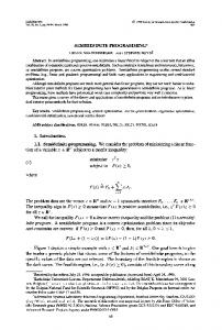
1 a1 a21 x1 b1       1 a1 a21   x2  =  b2  , 1 a1 a21 x3 b3 where a b are interval vectors of R3 .

1.6 1.4 1.2 1 0.8 0.6 4

6 8 x1

x3

x3

1 0.9

−5 −4 −3 −7 −6 x2

interval calculus

0.8

−4.5

x2

−4

ellipsoid calculus

Figure 1: Sets of confidence for an uncertain Vandermonde system. In Figure 5.3, we show the box of confidence for the solution, computed by direct application of interval algebra; the right-hand side plots shows the ellipsoid of confidence obtained by robust 17

semidefinite programming. We did not use elaborate algorithms to solve the problem via interval algebra, so the reader should not draw negative conclusions about it; rather, the instructive part is that the robust SDP method seems to behave well in this example.

5.4

Robust structural design

A typical problem of (static) structural design is to specify a mechanical construction capable best of all withstand a given external load. As a concrete example of this type, consider the Truss Topology Design (TTD) problem (for more details, see [1]). A truss is a construction comprised of thin elastic bars linked with each other at nodes – points from a given finite (planar or spatial) set. When subjected to a given load – a collection of external forces acting at some specific nodes – the construction deformates, until the tensions caused by the deformation compensate the external load. The deformated truss capacitates certain potential energy, and this energy – the compliance – measures stiffness of the truss (its ability to withstand the load); the less is compliance, the more rigid is the truss. In the usual TTD problem we are given the initial nodal set, the external “nominal” load and the total volume of the bars. The goal is to allocate this resource to the bars in order to minimize the compliance of the resulting truss. Mathematically the TTD problem can be modeled by the following semidefinite program: min τ s.t. " # τ fT (35) Pn (a) º 0, T f t b b i i i=1 i (b) t ∈ P ⊂ Rn+ , with design variables τ ∈ R and t = (t1 , . . . , tn ) ∈ Rn ; ti ’s are volumes of tentative bars. The data of the problem are • vectors bi ∈ Rm ; they are readily given by the geometry of the nodal set; • vector f ∈ Rm representing the external load; • a polytope P representing design restrictions like upper bound on the total bar volume, bounds on volumes of particular bars, etc. In reality, the external load f should be treated as uncertain element of the data; the traditional approach to treat this uncertainty is to consider a number of “loads of interest” f1 , . . . , fk and to optimize the worst-case, over this set of scenarios, compliance. Mathematically this approach is equivalent to replacing the LMI (35.a) (expressing the fact that τ is an upper bound on the compliance with respect to f ) by k similar constraints corresponding to f = f1 , f = f2 , . . . , f = fk . A disadvantage of the “scenario approach” is that it takes care just of a restricted number of “loads of interest” and ignores “occasional” loads, even small ones; as a result, there is a risk that the resulting construction will be crushed by a small “bad” load. An example of this type is depicted on Fig. 1. Fig. 1.a) shows a cantilever arm which withstands optimally the nominal load – the unit force f ∗ acting down at the most right node. The corresponding “nominal” optimal compliance is 1. It turns out, however, that the construction in question is highly instable: a small force f (10 times smaller than f ∗ ) depicted by small arrow on Fig. 1.a) results in a compliance which is more than 3,000 times larger than the nominal one. In order to improve design’s stability, it makes sense to treat the load as uncertain element of the data varying through a “massive” uncertainty set rather than taking just a small number of “values of interest”. From the mathematical viewpoint, it is convenient to deal with uncertainty set in the

18

form of an ellipsoid centered at the origin: n

o

f ∈ F = f = Lδ | δ ∈ D = {δ ∈ Rk : δ T δ ≤ 1} .

(36)

Problem (35) with perturbation set given by (36) is a particular case of full matrix uncertainty (32); according to Theorem 4.1, the robust counterpart of (35) – (36) is equivalent to an explicit semidefinite program; this program can be finally converted to the form min τ s.t. "

τI QT Pn T Q i=1 ti bi bi

#

º 0,

(37)

t ∈ P. (for details, see [1]). To illustrate the potential of the outlined approach, let us come back to the above “cantilever arm” example. In this example a load is, mathematically, a collection of ten 2D vectors representing (planar) external forces acting at the ten non-fixed nodes of the cantilever arm; in other words, the data in our problem is a 20-dimensional vector. Let us pass from the nominal problem (“a singleton uncertainty set F = {f }”) to the problem with F being a “massive” ellipsoid, namely, the ellipsoid of the smallest volume containing the nominal load f and a 20-dimensional ball B0.1 comprised of all 20-dimensional vectors (“occasional loads”) of the Euclidean norm ≤ 0.1kf k2 . Solving the robust counterpart (37) of the resulting uncertain SDP, we get the cantilever arm shown on Fig. 1.b).



 




 



 
      

   

  

     

                             a)

                                                                                                                                                                             b)

Figure 1. Cantilever arm: nominal design (left) and robust design (right) The compliances of the original and the new constructions with respect to the nominal load and their worst-case compliances with respect to the “occasional loads” from B0.1 are as follows: 19

Design nominal robust

Compliance w.r.t. f ∗ 1 1.0024

Compliance w.r.t. B0.1 > 3360 1.003

We see that in this example the robust counterpart approach improves dramatically the stability of the resulting construction, and that the improvement is in fact “costless” – the robust optimal solution is nearly optimal for the nominal problem as well.

6

Concluding Remarks

We have described a general methodology to handle deterministic uncertainty in semidefinite programming, which computes robust solutions via semidefinite programming. The method handles very general (nonlinear) uncertainty structures, and uses a special Lagrange relaxation (or, in a dual form, a “rank relaxation”) to obtain the approximate robust counterpart in the form of an SDP. The method is actually an extension of techniques that are well-known in several (apparently unrelated) areas, such as rank relaxations in combinatorial optimization, or Lyapunov functions in control. In the case of affine dependence, we can estimate the quality of the resulting approximation; in some other cases, the approximation is exact. Further work should probably concentrate on reducing the level of conservativeness as much as possible, while keeping the size of the approximate robust counterpart reasonable.

Acknowledgements Several people—especially the Editors of the handbook!

References [1] Ben-Tal, A. and Nemirovski, A. ”Robust Truss Topology Design via Semidefinite Programming”, Research Report # 4/95 (August 1995), Optimization Laboratory, Faculty of Industrial Engineering and Management, Technion – The Israel Institute of Technology, Technion City, Haifa 32000, Israel; to appear in SIAM Journal of Optimization. [2] Ben-Tal, A., and Nemirovski, A. ”Robust solutions to uncertain linear problems” – Research Report # 6/95 (December 1995), Optimization Laboratory, Faculty of Industrial Engineering and Management, Technion – the Israel Institute of Technology, Technion City, Haifa 32000, Israel; submitted to Operations Research Letters. [3] Ben-Tal, A., and Nemirovski, A. ”Robust Convex Programming” – Working paper (October 1995), Faculty of Industrial Engineering and Management, Technion – the Israel Institute of Technology, Technion City, Haifa 32000, Israel (to appear in Mathematics of Operations Research). [4] Boyd, S., El Ghaoui, L., Feron, E., and Balakrishnan, V. Linear Matrix Inequalities in System and Control Theory – SIAM, Philadelphia, 1994. [5] El-Ghaoui, L., and Lebret, H. ”Robust solutions to least-squares problems with uncertain data matrices” – SIAM J. Matrix Anal. Appl., October 1997.

20

[6] Falk, J.E. ”Exact Solutions to Inexact Linear Programs” – Operations Research (1976), pp. 783-787. [7] Goemans, M. X., and Williamson, D. P. ”.878-approximation for MAX CUT and MAX 2SAT” – In: Proc. 26th ACM Symp. Theor. Computing, 1994, pp. 422-431. [8] Golub, G.H., and Van Loan, C.F. Matrix Computations. John Hopkins University Press, 1996. [9] Hansen, E.R. Global optimization using interval analysis. Marcel Dekker, NY, 1992. [10] Lovasz, L. ”On the Shannon capacity of a graph” – IEEE Transactions on Information Theory v. 25 (1979), pp. 355-381. [11] Kosheler, M., and Kreinovitch, V. Interval computations web site http://cs.utep.edu/interval-comp/main.html, 1996. [12] Moore, E.R. Methods and applications of interval analysis. SIAM, Philadelphia, 1979. [13] Mulvey, J.M., Vanderbei, R.J. and Zenios, S.A. ”Robust optimization of large-scale systems”, Operations Research 43 (1995), 264-281. [14] Nesterov, Yu., and Nemirovski, A. Interior point polynomial methods in Convex Programming, SIAM Series in Applied Mathematics, Philadelphia, 1994. [15] Oustry, H., El Ghaoui, L., and Lebret, H. ”Robust solutions to uncertain semidefinite programs”, To appear in SIAM J. of Optimization, 1998. [16] Rockafellar, R.T. Convex Analysis, Princeton University Press, 1970. [17] Rohn, J. ”Systems of linear interval equations” – Linear Algebra and its Applications, v. 126 (1989), pp. 39-78. [18] Rohn, J. ”Overestimations in bounding solutions of perturbed linear equations” – Linear Algebra and its Applications, v. 262 (1997), pp. 55-66. [19] Singh, C. ”Convex Programming with Set-Inclusive Constraints and its Applications to Generalized Linear and Fractional Programming” – Journal of Optimization Theory and Applications, v. 38 (1982), No. 1, pp. 33-42. [20] Soyster, A.L. ”Convex Programming with Set-Inclusive Constraints and Applications to Inexact Linear Programming” - Operations Research (1973), pp. 1154-1157. [21] Van Huffel, S., and Vandewalle, J. The total least squares problem: computational aspects and analysis. – v. 9 of Frontiers in applied Mathematics, SIAM, Philadelphia, 1991. [22] Zhou, K., Doyle, J., and Glover, K. Robust and Optimal Control – Prentice Hall, New Jersey, 1995.

21