Sep 2, 2011 - operator (or a contractor) that reduces the size of the search domain . ..... Back, J., Yub, K. T., Seo, J. H. (2006.b). Dynamic observer error.
Preprints of the 18th IFAC World Congress Milano (Italy) August 28 - September 2, 2011
Robust state estimation for flat systems using set-membership techniques Ramatou Seydou, Tarek Raïssi, Ali Zolghadri
Bordeaux I University, IMS- lab, Automatic control group 351 cours de la libération, 33405 Talence cedex, FRANCE Abstract: Robust state estimation for a subclass of nonlinear systems is considered in this paper through a comparison of two methodologies. The comparison is based on modus operandi complexity, calculation time and interval observation quality. The first approach is based on a fundamental property of flat systems which states that the state of the system can be written as a function of the so-called flat outputs and their derivatives up to some order. Moreover, it is only assumed that the measurement noise and the disturbances are bounded without any additional information such as stationarity, uncorrelation or type of probabilistic distribution. Therefore, the interval state estimation is expressed as a set inversion problem which is solved using interval analysis. The second approach is based on coordinate transformation in order to obtain a partially linear cooperative presentation of the nonlinear system for which a closed-loop interval observer is designed. Both methods ensure to enclose the set of system states that is consistent with the model and the measurement noise bounds. The performance of each technique is discussed. Numerical examples are given throughout the paper to illustrate the performances of the proposed techniques. Keywords: Set-membership, state estimation, Set Inversion, Constraint Satisfaction Problem (CSP) Interval Observer, Cooperativity, Exact Linearization.
1. INTRODUCTION Since the precursor work reported in (Schweppe [1973]), many set-membership techniques for state estimation have been widely investigated to deal with approximate model structures and limited precision of computers; see (Alamo et al. [2008]) for a survey. Most of the literature is related to linear systems, and very few results are available to deal with nonlinear and changing dynamics ones. Usually, the admissible set of the state vector is approximated by several types of geometrical forms such as ellipsoids (Chernousko [2005]), zonotopes (Alamo et al. [2005]) or intervals (Jaulin [2009], Raïssi [2004]), whether the model is linear or not. This approach is basically different from the technique based on classical observers theory since the interval observers provide guaranteed lower and upper bounds for the estimate at any instant. In is paper, set-membership state estimation is investigated for an important subclass of nonlinear systems, the so-called flat systems; see (Fliess et al [1992]). Flatness property offers an easy way to parameterize the dynamical behavior of a system using “flat outputs”. Consider a nonlinear system described by: �� � ���� � ���. � � � �1� � ��� where � � �� is the state vector and the initial state belongs to a compact set �� � � � �� � , �� �. � � and � � � are respectively the measurement and the input. Without any loss of generality only Single Input Single Output (SISO) systems are considered here. Finally, �: � � �� � �� and Copyright by the International Federation of Automatic Control (IFAC)
: � x � � �! are two smooth vector fields and : �! � � is a smooth map. This paper presents two different approaches for robust state estimation of flat systems: Constraint Satisfaction based approach and Closed Loop Interval Observer. The first approach consists in formulating the state estimation into a Constraint Satisfaction Problem (CSP) where the state vector constitutes the variables set and a mapping, relating the state to the flat outputs and their derivatives is taken as the constraints. Branch and prune algorithms (Goldsztejn [2006], Benhamou and Granvilliers [2006], Neumaier [2004]), based on consistency, are used to compute an outer approximation of the solution set of the CSP. The second approach has been introduced initially in (Gouzé et al. [2000], Bernard and Gouzé [2004], Moisan et al. [2009]) for a subclass of nonlinear systems described by �� � "� � #�. � �2� where the nonlinearity is captured in the function #�. � which depends on the output and/or the state vectors. The observer gain is chosen such that the observation error is cooperative (Smith [1995]). In this case, two suitable point observers are designed to compute a lower and an upper bound for the domain of the state vector. This approach has been extended in (Raïssi et al. [2010]) to a large class of nonlinear systems based on a LPV (Linear Parameter-Varying) transformation of the original nonlinear model. The main limitation of the interval observers proposed in (Gouzé et al. [2000]) is that most of nonlinear systems cannot be described by �2�. In this paper, we will show that such a drawback could be avoided for flat systems through a nonlinear change of coordinates
7450
Preprints of the 18th IFAC World Congress Milano (Italy) August 28 - September 2, 2011
based on the Exact Linearization (Isidori [1985]). Nevertheless, the methods proposed in (Gouzé et al. [2000]) cannot be applied for the obtained linear form. Thereby, a second change of coordinates is necessary in order to obtain an interval observer. Note that the convergence of both bounds can be tuned such that the estimated interval width tends to zero in the ideal case or, at least, tends to a small value for practical cases. This approach is fundamentally different from the first one since the convergence of CSPbased estimators depends only on the tolerance chosen for the branch and prune algorithm. In addition, the evaluation of the derivatives of the flat outputs up to a given order is needed for CSP observers. The paper is structured as follows. Section 2 recalls the basic definitions for nonlinear observability, flatness notions and interval analysis. In section 3, the CSP observer technique is detailed and illustrated through an example that will also be used in section 4 to support the closed-loop interval observer approach. The performance of both methods is discussed and finally some concluding remarks are given. 2. PRELIMINARIES Flatness and observability Definition 2.1 (Rouchon [2008]): System �1� is said to be flat with a flat output if and only if one can describe the system states and input ��, �� only from the flat output and a finite number of its derivatives, i.e.: �3� � � %& , � , … , � � ( )*+ � � ,� , � , … , � -.� � where % and , are respectively a smooth vector field and a map. A system is also said to be flat if its relative degree 0 � *, (Waldherr et al. [2007]). Definition 2.2 (Hedrick and Girard [2005]): Nonlinear observability is intimately tied to the Lie derivative. The Lie derivative is the derivative of a scalar function along a vector field. Let �: �! � �! be a vector field in �! and : �! � � a smooth scalar function. Then the Lie derivative of with respect to � is: 34 34 1� � 2 . � � . � � ∑!:;. . �9 �4� 35
378
With 1=� � , and 1>� � 1�1>?. � �. System �1� is said to be locally observable if and only if the following rank condition is fulfilled: +@A B,C)* D ���, +1� ���, … , +1�
�!?.�
���EF � *
where * is the system dimension. From its definition, a flat system is obviously observable.
�5�
Interval tools A real interval �)� � �), )� is a connected and closed subset of �. The set of all real intervals of � is denoted by H�. Real arithmetic operations are extended to intervals (see Moore [1966], Hansen [2004]). Consider an operation o J K�; M; N ; /P and �)�, �Q� two intervals, then: �)�R�Q� � KS R | S J �)�, J �Q�P. The width of an interval �)� is defined by U�)� � ) M ) and its midpoint by A@+�)� � �) � )�/2. Inclusion functions Let �: �! � �V ; the range of the function � over an interval
vector [x] is given by: � ����� � K� ��� | � J ���P An interval function ���: �! � �V is an inclusion function for � if: W��� J H�! , � ����� � �� ������. An inclusion function of � could be obtained by replacing each occurrence of a real variable by its corresponding interval and by replacing each standard function by its interval evaluation. Such a function is called the natural inclusion function. In practice, the inclusion function is not unique and depends on the formal expression of . When the manipulated intervals are not large, the centered form could give better results than the natural one. We can now present the first state estimation technique based on Constraint Satisfaction applied to flat systems. Since the derivatives of the flat output are required, a High Order Sliding Mode differentiator is used in the sequel because of its robustness properties (Levant [1998]). 3. CONSTRAINT SATISFACTION BASED OBSERVER The numerical observer presented in this section is based on the form �3� which can be rewritten as (Jaulin et al. [2009]):
�6� X � & , �.� , … , � � ( � Z�[� � \��S, ��Y � The function Z can be obtained by successive derivatives of the flat output with respect to time. The goal is to estimate the state vector � based on the expression �6� at the sampling times ^_ . Denote respectively by ` a , ba , the domains of � and X at ^_ . Note that if no prior information about the domain of � is available, we can select ` a �� M ∞, �∞�. Thus, the state estimation method consists in computing all the values of � satisfying: Y
Xa � Z�&� a , �_ ( � � d Xa f ba �7� �a f `a The system �7� is called a Constraint Satisfaction Problem (CSP). The idea is to remove parts of the search domain ` a for the model states that are inconsistent with the measured data and their derivatives up to order C. The ideal case is to keep only the values that are consistent with the data. However, this task is harder and we look only for an enclosure of the solution set. Denote by ha the searched solution set at ^_ . An outer enclosure of ha could be computed by interval analysis. The idea is to use an interval narrowing operator (or a contractor) i that reduces the size of the search domain ` a . This operator removes some parts from ` a that do not contain a solution for �7�. It satisfies the soundness and completeness properties (Neumaier [2004]): i�` a � � ` a and C�` a � j ha � ` a j ha . Most narrowing operators use interval propagation techniques that are based on an interval extension of the local Waltz filtering (Waltz [1972, 1975], Chun [1999]). Usually, the narrowing process is not optimal and the contracted set ` ka l i�` a � still contains inconsistent values. In such a case, the domain ` ka is split along its widest side. Both halves are then subjected to the same narrowing process. This procedure ends when the generated domains have reached a smallest tolerable size m fixed by the user. Finally, a list hna containing consistent state boxes is obtained; it satisfies: ha � hna . Since
7451
e
Preprints of the 18th IFAC World Congress Milano (Italy) August 28 - September 2, 2011
the map Z is assumed to be smooth, the enclosure hna converges towards the exact solution set ha when the tolerance m tends to 0 which means that the convergence of the observer is governed by m. Furthermore, the estimator requires the evaluation of the derivatives up to an order C of the noisy measurements. This task is achieved in this paper using a High Order Sliding Mode (HOSM) differentiator. Besides the control context, sliding mode techniques are also used for observation, fault detection (Rolink et al. [2006]) and differentiation (Levant [1998, 2001]). Let ��^� be the signal to be differentiated and o= , o. … o! some estimates for the signal ��^� and its derivatives. ��^� � �= �^� � p�^� and p�^� is a bounded Lebesgue-measurable noise with unknown features and an unknown base signal �= �^� with the nth derivative having a known Lipschitz constant C > 0. The nthorder HOSM differentiator is given by: ! ��^�|!-.
,@w*&o= M ��^�( � o. t o�= � u= , u= � Mv= |o= M !?. r r o�. � u. , u. � Mv. |o. M u= | ! ,@w*�o. M u= � � ox … r !?: r o�: � u: , u: � Mv: |o: M u:?. |!8-. ,@w*�o: M u:?. � �8� �o :-. s … r r o�!?. � u!?. , . r r u!?. � Mv!?. |o!?. M u!?x |x ,@w*�o!?. M u!?x � � o! q o�! � Mv! ,@w*�o! M u!?. � Coming back to the problem at hand, the main assumption in this paper is that the measurement error p is bounded with a prior known bound p. Thus, domain is given by: z � V M p, V � p�
where V is the measurement. The derivatives are estimated via the nth-order HOSM differentiator �8�. It has been proved in (Levant [2001]) that the ith derivative best estimate
accuracy is proportional to ){{ � |: . i . p ,@ � 0, … , * when the Lipschitz constant of the nth derivative of the clear-off-noise signal is bounded by a certain constant i �:� and |: 1. Hence, the derivative domain is: �:� z �
M �:� �:� ){{,
� ){{� where
is the derivative estimate. For easy reference, the main steps of the state estimation are summarized in the following algorithm. 8 }~
}~8 � }~
�
Algorithm CSP Estimator �Inputs: �^: �, i�1..N, I.D*: I.D* �� � �� 1.
2.
Flatness modeling �eq. 6�
For i�1 to N do,
Estimate the derivatives
� �
, q�1,2..p �eq. 8�
The CSP observer methodology is illustrated through a numerical example. Consider the following system: S�. � p 7¤ � S� � S. � p 7¤ � � d x S� ¥ � S. M Sx � S¥
The goal is to estimate S. and Sx .
S � MS§ ¥ � M § t . r Sx � M�S§ ¥ � S� ¥ � � M� § � � � � S � s ¥ 7� © « r � � � M 7©ª � M �¬§~¬�� q ¨¤ �¨§ ª ~¨� ª �
Step 1. It is easy to prove that:
which means that the system �9� is flat.
Step 2. A third order HOSM differentiator is used to estimate the first and second derivatives of the output . The second derivative Lipschitz constant i is taken as i=1 (the measurable output function is a cosine function) and |: � | �� 1.1 1 . .
x
t o�= � u= , u= � M3i ¥ |o= M ��^�|¥ ,@w*&o= M ��^�( � o. .
.
s o�. � u. , u. � M1.5i x |o. M u= |x ,@w*�o. M u= � � ox qo�x � M1.1i,@w*�ox M u. �
�
Since S¥ is the measured flat output, we do not need to estimate it and its estimate enclosure is given by �o= M p, o= � p�, where p � 0.001 and o= is the measurement estimate. The expression of S. is simple and derives from the flat output second derivative: S. � M § .
Based on the accuracy ){{ expression, @ � 2 here, we have:
){{x � 1.1 N �0.001�
� 0.11 and
){{. � 1.1 N �0.001�
� 0.011
¤~¤ ¤~
S. � �M §® � z �Mox M ){{x , Mox � ){{x �.
The first derivative of � S¥ is also necessary to estimate Sx using the expression Sx � M� § � � �, thus: ¤~ ¤~
which means that: �® z �o. M ){{. , o. � ){{. �. Finally, the system �10� can be rewritten as: � , �, §�Y � � S¥ , S. M Sx , MS. �Y
�11�
��S.= �, �Sx= ��Y � ��M2, 2�, �M2, 2��Y
and assume that the tolerance is chosen as: m � 0.2.
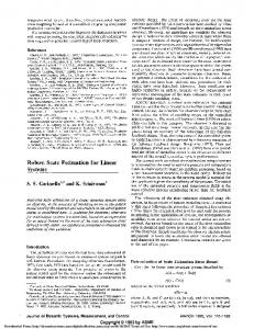
x1 signal and its estimated bounds (noise at t=1s, step amplitude=1e-3)
1.5
Lower bound Upper bound x1 signal (simulation)
1
Solve CSP to obtain ���^: �� �eq. 7�
Example
�10�
The prior search domain for S. and Sx is:
Estimate the bound acc and construct the domains of �^: � and �:� �^: �
* I.D: Initial search Domain
�9�
0.5
0
-0.5
-1
Figure 1.a: The bounds of S. estimated by the CSP observer -1.5 0
7452
1
2
3
4
5
6
7
8
9
10
Preprints of the 18th IFAC World Congress Milano (Italy) August 28 - September 2, 2011
�� � ���� � ���. � � � �14� � É��� has a relative degree * at � ¯ . This lemma ensures that flat systems could be transformed into a partial linear form that simplifies the design of nonlinear observers. Once the system is transformed into �13�, the second issue is about designing an interval observer with two bounds described by two similar dynamical systems. Basically, the proposed observer will be a Luenberger-like one with the gain Ê as a tunning parameter for the convergence.
x2 signal and its estimated bounds (noise at t=1s,step amplitude =1e-3) 1.5
1
0.5
0
-0.5
-1 Lower bound Upper bound x2 signal (simulation)
-1.5 0
1
2
3
4
5
6
7
8
9
10
Figure 1.b: The bounds of Sx estimated by the CSP observer Time (s)
The bounds of the state variables are plotted in figures 1.a and 1.b. The set-membership approach ensures that the actual trajectory belongs to the estimated bounds. In addition, the signal domain thickness is an indicator of the estimation quality. The convergence of this observer is ensured by the tolerance m, that increases the computation time. What can be an alternative to this problem is the design of an interval observer. 4. CLOSED-LOOP INTERVAL OBSERVER 4.1 Partial linear formulation The idea here is to linearize the system (1) in order to design an observer with a linear observation error. Several linearization approaches exist among which Exact Linearization Via Feeback (Isidori [1985]). Suppose that (1) has a relative degree 0 � * at the neighborhood of a point � � � ¯ . Then, as shown in (Isidori [1985]), the change of coordinates � � %��� defined by:
��� ±. ��� µ ¸
��� · 1 ��� ± %��� � ° x ² � ´ � �X … ´ !?.… · ±! ��� ³1� ���¶
�12�
transforms the nonlinear system �1� into a partially linear one described by: o�. � ox o�x � o¥ = = … » ½ � D » E �� � � ¹X� � "X � º¼�X� ¾�X� o�!?. � o! s � iX ro�! � Q�X� � )�X�� � o. q t r
where
0 1 0 … 0 … 0 Á» 0 1 Å " � À» » 0  »Ä  » » » 1 … 0 ¿0 0 0 Ã
and
i � �1 0 … 0�.
�13�
Moreover,
X¯ � ±�� ¯ � and at all X in the neighborhood of ÆÇ , the function )�X� is nonzero. Note that the linearization �13� is ensured by the following lemma. Lemma 4.1 (Isidori [1985]): The State Space Exact Linearization problem is solvable if and only if there exists a neighborhood È of � ¯ and a real-valued function É���, defined on È such that the system
4.2 Interval observer design In the following, two Luenberger-based observers are designed based on the partial linear form �13� to estimate reliable lower and upper bounds for the actual state trajectory of �1�. Firstly, let us recall some results which will be useful to introduce the main result summarized in the proposition 4.4. Definition 4.2.1 Given a system described by �1� where the Ì initial state � � belongs to �� � , �� �, @. p. � � Ë � � Ë �� , for which the system has bounded solutions. A dynamical system described by: Y Î &�, �, ^( &�, �( � Í � ¹ �15� Y Ï��^= �, ��^= �Ð � �� � , �� �Y Î is a smooth vector field, is called an interval where Í observer for (1) if: 1. there exists a solution for �15� for all ^ 0; 2. for any initial condition satisfying� � Ë � � Ë �� , the solution of �15� verifies: M∞ Ñ ��^� Ë ��^� Ë ��^� Ñ �∞. Usually, the design of �15� is based on the theory of cooperative systems which are recalled in the following definition. Definition 4.2.2 (Smith [1995]): A dynamical nonlinear system described by �� � ���� is said to be cooperative over a domain ��� if all off-diagonal terms of f Jacobian matrix are non-negative over ���, ie: 3 �_ ��� 0 W @ Ò Ó, ^ 0 ��Ô� J ��� �16� 378
For linear systems, �16� leads to the following proposition: Proposition 4.3 (Gouzé et al [2000]) Given a linear system of the form: �17� �� � "� � É�^�; ���� � � � where " is cooperative �):_ 0, @ Ò Ó� and É�^� 0.If � � � then ��Ô� �, W ^ 0. In the following, assume that the maps )�. � and Q�. � are Lipschitz continuous which constitutes a standard assumption in classical observers design (Aboky et al. [2002]). Moreover, by the definition of flat systems the system �13� is observable. Then, there exists a gain L such that: X� � �" M Êi�X � )�X�� � Q�X� � Ê �18� is a classical (point) observer for �13�. Furthermore, by assumption, the functions ) and Q are assumed bounded, then the equation �18� could be rewritten as: X� � "Õ X � U �19� where "Õ � " M Êi )*+ U � )�X�� � Q�X� � Ê . Satisfying simultaneously both stability and cooperativity for the matrix "Õ is quite unfeasible with the same gain L in the z
7453
Preprints of the 18th IFAC World Congress Milano (Italy) August 28 - September 2, 2011
basis. Therefore, the interval observer proposed in (Mazenc and Bernard [2010]) for Linear-Time Invariant systems could be extended to flat systems using �19�. A new change of coordinates is then performed in order to work in a basis Ö offering stability and the cooperativity property to the system (19). This is done via the jordanization of the matrix "Õ . Finally, the proposed interval observer is given in the following proposition: Proposition 4.4: Consider the linear time-invariant change of coordinates defined by: Ö � ×X and Ø � ×"Õ × ?. , where × is the transition matrix. It then transforms the system (19) into the cooperative system: �t Ö � ØÖ � �×[� rÖ�? � ØÖ? � �×[�? � �20� ? s ÖÙ � max�×�XÙ , XÙ �� r ? ? q ÖÙ � min�×�XÙ , XÙ �� ? where Ö and Ö are respectively the lower and the upper bounds of the state vector in the Ö basis. The bounds of X and � would then be derived from an interval evaluation of the maps × ?. Ö and %?Ì �X� using interval analysis.
Proof: It takes two steps to prove that �20� is an interval observer for �1�. We must first prove the error positivity and then establish the convergence. Step 1. Since )�. � and Q�. � are assumed bounded, we can write: )&X, X( Ë )�X� Ë )&X, X( and Q&X, X( Ë Q�X� Ë Q&X, X( and consequently w is also bounded and Lipschitz continuous. Thus, one can write in the Ö basis: �×[�? Ë �×[� Ë �×[�- . �21� Denote by ÖÚ- � Ö- M Ö and ÖÚ? � Ö? M Ö respectively the upper and the lower error. The aim is to prove that ÖÚ- � and ÖÚ? Ë � at any time t. The dynamics of Ö- is described by: ÖÚ-� � Ø. ÖÚ- � �×[�- M �×[� �22� From �21� one can easily deduce that ��×[�- M �×[�� is always positive and the matrix Ø cooperativity ensures the positivity of ÖÚ- . A similar methodology leads to the negativity of the lower bound. Step 2. Since a(.) and b(.) are assumed to be Lipschitz continuous and bounded functions, there exists Û z �!- such that �×U�- M �×U� Ë Û W^ 0. Furthermore, the gain L is chosen such that the matrix J is cooperative and stable. Thus, based on the lemma 1 in (Moisan and Bernard [2006]), the observation error (18) admits an upper bound MØ?. Û.
Example xÜÝ� �
� Consider again the system �9� and assume that � � M ¨¤ . For simulation purposes, the initial conditions have been chosen as: �S.= , Sx= , S¥= �Y � �1, 1, 1�Y . Flatness has already been proved and this property implies a relative degree 0 � * � 3. Subsequently, we can proceed to the linearization step with the following change of coordinates: o. � ��� � S¥ ¹ ox � 1� ��� � S. M Sx � o¥ � 1x� ��� � MS.
This implies that the state space representation �13� is defined by the matrices: 0 1 0 " � º0 0 1½ , i � �1 0 0� 0 0 0 and a “conventional observer” could be built as: X� � �" M Êi�X � ¼�X� � ¾�X�. � � Ê � � � iX where the gain Ê � �Þ. , Þx , Þ¥ �Ô is computed via the following pole assignment: ß � �M1, M2, M4�Y . The interval observer is designed based on �20� where the initial conditions can be deduced from the last two lines of �20� with: X� � ��0.8, 1.2�, �M0.2, 0.2�, �M1.2, M0.8��Y The main assumption on the bounds is: p � 0.001. Moreover, gaussian noise (CRUp0 � 1p M 4) is added to the measurement. x1 signal and its estimated bounds (gaussian noise on the measured output x3)
2 Lower bound Upper bound x1 signal (simulation)
1.5
1
0.5
0
-0.5
-1
-1.5
-2 0
Figure 2.a: The actual value of S. and estimated bounds 1
2
3
4
5
6
7
8
9
10
Time (s)
x2 signal and its estimated bounds (gaussian noise on the measured output x3)
4
Lower bound Upper bound x2 signal (simulation)
3
2
1
0
-1
-2
-3
-4 0
Figure 2.b: The actual value of Sx and estimated bounds 1
2
3
4
5
6
7
8
9
Time (s)
From figures 2.a and 2.b, it can be seen the pessimism induced by this method. Actually, it is more important than in figures 1.a and 1.b because of the two extra steps (reciprocal function to get X from Ö and reciprocal function to get � from X) between the interval observer in the second basis (Ö� and the estimates in the original basis (�). 5. CONCLUDING REMARKS Robust state estimation for flat systems has been studied in this paper through two set-membership methods: Constraint Satisfaction based Observer and Interval Observer. It is shown that as far as we restrict the study to flat systems, the first method gives better estimation performance; the price to pay is higher computational time. Actually this computing time increases exponentially with the state dimension, in addition the number of bisections also increases with the �27� tolerated precision, i.e when m becomes small. The Interval Observer method also offers interesting results and requires
7454
10
Preprints of the 18th IFAC World Congress Milano (Italy) August 28 - September 2, 2011
less computation time however the major problem remains the choice of the observer gain L. In this paper, this choice was made after several trials without any analytic analysis. Finally, this study only deals with systems having a relative degree 0 � *. To avoid this restriction, for the Interval Observer method, the linearization could be performed using techniques such as System Immersion (SI) or Dynamic Observer Error Linearization (DOEL) (Back et al. [2006.a, 2006.b]). Note that the Constraint Satisfaction based observer technique can also be used but it becomes harder to implement since the flatness property is no longer preserved. References: Aboky C., Sallet G., Vivalda, J.C. (2002). Observers for Lipschitz nonlinear systems. International Journal of Control 75, 204-212. Alamo T., Bravo J. M. Redondo, M. J. and Camacho E. F. (2005). Guaranteed state estimation by zonotopes. Automatica 41, 1035-1043. Alamo T., Bravo J. M. and Camacho E. F. (2008). A setmembership state estimation based on DC programming. Automatica 44(1), 2216-224. Back, J., Seo, J. H. (2006.a). An algorithm for system immersion into a nonlinear observer form: SISO case. Automatica 42, 321-328. Back, J., Yub, K. T., Seo, J. H. (2006.b). Dynamic observer error linearization. Automatica 42 (2006) 2195 – 2200 Benhamou, F. and Granvilliers, L. (2006). Continuous and interval constraints. In P. van Beek F. Rossi and T.Walsh. Handbook of constraint programming, 571-604. Elsevier. Bernard, O., Gouzé J. L. (2004). Closed loop observers for uncertain biotechnological models. Journal of Process Control, 14(7), 765-774. Chernousko, F. L. (2005). Ellipsoidal state estimation for dynamic systems. Nonlinear Analysis 63(5-7), 872-879. Chun, A. H. W. (1999). Waltz filtering in java with JSolver. Proceedings of PA Java99, The Practical Application of Java, London, UK. Fliess, M., Lévine, J., Martin P., Rouchon P. (1992). Sur les systèmes non linéaires différentiellement plats. Elsevier, Paris, FR. Fogel, E. and Huang, Y. H. (1982). On the value of information in system identification–bounded noise case. Automatica 18(2), 229 - 238. Goldsztejn, A. (2006). A branch and prune algorithm for the approximation of non-linear AE-solution sets. Proceedings of the 2006 ACM Symposium on Applied Computing. Dijon, FRANCE. Gouzé, J. L, Rapaport, A., Hadj-Sadok, M. Z. (2000). Interval observers for uncertain biological systems. Elsevier Ecological Modelling 133, 45-56. Hansen, R. E. (2004). Global optimization using interval analysis, second edition. CRC. Hedrick, J. K and Girard, A. (2005). Control of nonlinear dynamic systems: Theory and applications. Controllability and observability of Nonlinear Systems. Isidori, A. (1985, 1989). Nonlinear control systems. 156- 172. Pringer-Verlag, Berlin, DE. Jaulin, L. (2009). Interval contractors and their applications. Ecole JN-MACS. Jaulin, L., Sliwka, J., Le Bars F., Xiao, K. (2009). Combining flatness with of interval analysis for state estimation. Journée MEA Paris. Levant, A. (1998). Robust exact differentiation via sliding mode technique. Automatica 34(3), 379-384.
Levant, A. (2001). Higher order sliding modes and arbitrary-order exact robust differentiation. Proceedings of the European Control Conference. Mazenc, F., Bernard, O.(2010). Time-varying interval observers for linear systems with additive disturbances. 8th IFAC Symposium on Nonlinear Control Systems. Bologna, Italy. Milanese, M., Norton, J., Piet-Lahanier, H., and Walter E. (1996). Bounding approaches to system identification. Plenum, New York. Moisan, M., Bernard O. (2006). Robust interval observers for uncertain chaotic systems. In 45th IEEE Conference on Decision and Control, San Diego, USA. Moisan, M., Bernard, O., Gouzé, J. L. (2009). Near optimal interval observers bundle for uncertain bioreactors. Automatica 45(01), 291-295. Moore, R. E. (1966). Interval analysis. Prentice Hall, Englewood Cliffs, NJ, USA. Neumaier, A. (2004). Complete Search in Continuous Global Optimization and Constraint Satisfaction. Acta Numerica. Cambridge: University Press. Raïssi, T., Ramdani, N, Candeau, Y. (2004).Set membership state and parameter estimation for systems described by nonlinear differential equations. Automatica,40(10),1771 1777. Raïssi, T. (2004). Méthodes ensemblistes pour l’estimation d’état et de paramètres. PhD thesis. Raïssi, T., Videau, G. and Zolghadri, A. (2010).Interval observer design for consistency checks of nonlinear continuoustime systems. Automatica 46(3), 518-524. Rolink, M., Boukhobza, T., Sauter, D. (2006). High order sliding mode observer for fault actuator estimation and its application to the three tanks benchmark. Rouchon, P. (2008). Systèmes différentiellement plats. JNCF, CIRM. Schweppe, F. (1973). Uncertain dynamic systems: modelling, estimation, hypothesis testing, identification and control. Prentice Hall, Englewood Cliffs, NJ, USA. Smith, H. L. (1995). Monotone dynamical systems: an introduction to the theory of competitive and cooperative systems. Mathematical surveys and monographs 41. Providence, RI. Vasiljevic, L. K., Khalil, H. K. (2008). Error bounds in differentiation of noisy signals by high-gain observers. Elsevier, Systems & Control Letters 57, 856–862. Waldherr S., Zeitz M., (2007). Conditions for the existence of a flat input. Unpublished version, International Journal of Control. Waltz, D. L. (1972). Generating semantic descriptions from drawings of scenes with shadows. Technical Report, AITR-271, MIT Artificial Intelligence Laboratory, Cambridge, MA. Waltz, D. L. (1975). Understanding line drawings of scenes with shadows. In The Psychology of Computer Vision, McGraw-Hill, 19-91.
7455