Robust task scheduling in non-deterministic heterogeneous ... - LaBRI

Robust task scheduling in non-deterministic heterogeneous computing systems Zhiao Shi Innovative Computing Lab Department of Computer Science University of Tennessee Knoxville, TN 37996, USA [email protected]

Emmanuel Jeannot Innovative Computing Lab and LORIA INRIA, Nancy University, CNRS Campus Scientifique - BP 239 54506 Vandœuvre-l`es-Nancy Cedex, France [email protected]

Jack J. Dongarra Innovative Computing Lab Department of Computer Science University of Tennessee Knoxville, TN 37996, USA and Computer Science and Mathematics Division Oak Ridge National Laboratory , Oak Ridge, TN 37831, USA [email protected]

Abstract The paper addresses the problem of matching and scheduling of DAG-structured application to both minimize the makespan and maximize the robustness in a heterogeneous computing system. Due to the conflict of the two objectives, it is usually impossible to achieve both goals at the same time. We give two definitions of robustness of a schedule based on tardiness and miss rate. Slack is proved to be an effective metric to be used to adjust the robustness. We employ ǫ-constraint method to solve the bi-objective optimization problem where minimizing the makespan and maximizing the slack are the two objectives. Overall performance of a schedule considering both makespan and robustness is defined such that user have the flexibility to put emphasis on either objective. Experiment results are presented to validate the performance of the proposed algorithm. Keywords: DAG, task scheduling, robustness, heterogeneous system, genetic algorithm

1

Introduction

Efficient scheduling of application tasks is critical to achieving high performance in parallel and distributed systems. The problem can be stated as assigning tasks of a par-

allel application to distributed computing systems so that the schedule length, or makespan can be minimized. A variety of application models exist in the literature of task scheduling. For example, a parallel application with data dependencies among subtasks is usually modeled as a Directed Acyclic Graph (DAG). Problem of scheduling this type of application is usually NP-hard. Thus, various of heuristic approaches have been developed to solve the problem [1, 16, 18, 22, 23, 24, 28]. The most studied heuristic methods are so called list scheduling algorithms [18]. Other types of heuristics include clustering algorithms [16], duplication based algorithms [17] and guided random search methods such as genetic algorithm and simulated annealing [15]. Although differing in the way of modeling target computing systems (e.g. heterogeneous vs. homogeneous processors, with vs. without communication cost etc.), the methods mentioned above are all based on a deterministic model. In this model, all information about the tasks (durations) and relationships among them (dependencies in the DAG) are supposed to be known by the scheduling algorithm a priori. It is assumed that task execution time can be estimated and does not change during the course of execution. However, this assumption does not usually hold in a real computing environment. In many cases, the actual execution time of a task is different from the expected one. The problem can be dealt with in several ways. For exam-

ple, dynamic scheduling algorithm assigns each ready task according to the current status of the resource environment aiming to avoid the inaccuracy of execution time estimation. Another possible approach is to judiciously overestimate the execution time of each task according to its variability hoping that the real execution time will not exceed the estimated one. Thus, the schedule will perform as well as expected. However, this approach could result in a low resource utilization. In this paper, we take on the challenge by using static algorithm to find schedules less vulnerable to the non-deterministic nature of the task execution time, i. e. more robust. As with other deterministic scheduling algorithms, our scheduler is fed with the expected task execution times. We then define a metric called slack for a schedule based on the slack of individual task. The slack of a task represents a time window within which it can be delayed without extending the makespan and it is intuitively related to the robustness. of the schedule. Larger slack tends to absorb the task execution time variance with little delay. Next, we develop a genetic algorithm based heuristic to generate schedules that are more robust compared with schedules obtained by another popular heuristic called HEFT [24]. Genetic based task scheduling algorithms [8, 15, 25, 26] normally use the makespan as their objective function. However, in order to take into account both the robustness and makespan, it is necessary to include the slack in the objective function. Unfortunately, slack and makespan are two conflicting metrics as shown in section 5.1. Optimizing only makespan will result in schedules with small slack thus less robust to task execution time variability. Conversely, optimizing slack alone tends to give robust schedule but with large makespan. To handle this multi-objective optimization problem (MOOP) [10], we employed the ǫconstraint method. In this method, an upper bound of expected makespan is given by ǫ · MakespanHEF T . The scheduling algorithm tries to find the schedules with maximal slack without exceeding the specified upper-bound. Although the robustness of a schedule is a desirable property and conceptually easy to perceive, it is difficult to measure quantitively. There are several attempts to define it according to different perspectives of the problem [2, 3, 12, 19]. We give two new measures of robustness. based on tardiness and miss rate in this work. Results show that the proposed algorithm can effectively trade off makespan for robustness. The rest of the paper is organized as follows: In the next section, we provide some related work about robust task scheduling. In Section 3 the robust task scheduling problem is described. Section 4 presents a genetic algorithm based approach to solve the bi-objective optimization problem. We show some experimental results in Section 5. The paper concludes in Section 6.

2

Related work

A large amount of research has been carried out in dealing with uncertainty in task scheduling, aiming to make schedules more robust to the uncertainty. In [9], the authors conduct a survey about some of the research performed within the Artificial Intelligence and Operations Research communities. The survey shows that very little understanding or characterization of dynamic, uncertain scheduling environments is available. Many issues such as how to strike a balance between robustness and other scheduling performance metrics need be addressed. Chiang and Fox [7] study the job shop scheduling problem with deviations in scheduled operation time due to the uncertainty of machine breakdown. Their idea is to add slack to protect the job from the need of rescheduling. The uncertain processing time was modeled with several types of fuzzy numbers. Leon et.al. [19] redefine the evaluation function of a schedule to include the robustness. A number of robustness measures are developed and evaluated in the context of job shop scheduling. The uncertainty in their model is due to disruption. The authors define the slack for each job as the amount of room it has to shift within the schedule without breaking any constraint nor extending the makespan. Experiments show that the mean job slack was a good predictor of average schedule delay. In [20, 21], the problem of scheduling tasks with precedence constraint and communication disturbances is studied. The authors propose a partially on-line scheduling algorithm based on critical paths to deal with the possible disturbances. An off-line schedule is generated first based on estimation of communication time. Then a partial order is computed by adding precedences between tasks assigned to the same processor according to some rules. At execution time, a complete schedule considering the static schedule and partial order can be obtained use some specified policy. Their model only considered uncertainty of communication delay. In addition, processors were assumed to be identical. Gupta et.al. [14] consider the problem of scheduling precedence task graph with disturbances in computation and communication times. Their solution to the problem is to add some extra edges to protect the off-line schedule from performance degradation. The purpose of adding so called “pseudo-edges” is to wait for high priority tasks to become ready in order to avoid situations where high priority tasks cannot be executed according to the static schedule because of disturbances. Robust scheduling of meta-programs is investigated in [5]. The authors give two measures of robustness. The number of critical components within a schedule is a good indicator of the robustness of the schedule. The fewer critical components, the more robust the schedule. Another measure of robustness proposed is the entropy of the schedule which is based on the probability of an exe-

cution path that will become critical. However, determining this probability is non-trivial. The authors argue that robustness analysis can improve the quality of the schedule by showing that the number of safer components is increased. Nevertheless, the performance of generated schedule is not examined within the real computing environment. In this paper, we compare the performance of schedules obtained using our algorithm with those generated by another heuristic (HEFT) in the real resource environment. Furthermore, we propose two more expressive definitions of the robustness of a schedule.

44

44

66

55

33

22

33

22

77 88

88

(d )

(a ) P1 PP11

1

2

4

PP22

3

P2

Robust task scheduling problem

66

55

77

PP33

3

11

11

PP44

5

8 6

P3

7

P4

(b )

In this section, we present a formulation of robust scheduling a task graph.

3.1

Basic Models

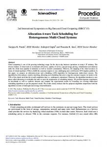
A task graph is defined by G = (V, E), where V = {v1 , v2 , ..., vn } is the set of n tasks. E is the set of directed arcs or edges between the tasks that maintain a partial order among them. The partial order introduces precedence constraints, i. e. if edge ei,j ∈ E, then task vj cannot start its execution before vi completes. vi is an immediate predecessor of vj and vj is an immediate successor of vi . A node with no predecessor is called an entry node and a node with no successor is called an exit node. Matrix D of size n × n denotes the communication data size, where di,j is the amount of data to be transferred from vi to vj . A heterogeneous multiprocessor computing system is composed of a set P = {p1 , p2 , ..., pm } of m fully connected processors. We assume that all inter-processor communications are performed without contention and computation can be overlapped with computation. To each task vi , there is an associated vector representing its minimal duration on each processor, i. e., the best case execution time (BCET ). B is an n × m matrix where bi,j gives the best case execution time of task vi on processor pj . Furthermore, we assume that random variables ci,j are independent of each other. The data transfer rates between processors are represented by matrix T R of size m × m. Intra-processor communication cost is assumed to be zero. In this paper, we do not consider the variation in data transfer rates. A schedule represents the assignment of tasks onto processors. It is denoted as a vector s = {s1 , s2 , ..., sm }, where si = {(vj1 , vj2 ), ..., (vjki −1 , vjki )} denotes the task execution order on processor i. ki is the number of task nodes assigned to processor i. Fig. 1 illustrates an example of task graph, a multiprocessor system and a schedule. The schedule shown in Fig. 1(c) can be denoted as {{(v1 , v2 ), (v2 , v4 )}, {(v3 , v5 ), (v5 , v8 )}, {(v6 , v7 )}, φ}.

0

2

4

6

8

(c )

Figure 1. (a) An example task graph (b) A multiprocessor system (c) A schedule (d) A disjunctive graph of (a) with schedule (c)

Definition 3.1. Given a task graph G = (V, E) and a schedule s = {s1 , s2 , ..., sm }, we denote by Gs the disjunctive graph of G under Sschedule s as: Gs = (Vs , Es ), where Vs = V, Es = E E ′ . E ′ is the set of disjunctive edges. E ′ = {ei,j |ei,j ∈ / E, ∃k ∈ {1, ..., m}, s.t.(vi , vj ) ∈ sk }. The data size matrix associated with Gs , Ds is: ( 0 ∃k ∈ {1, ..., m}, s.t.(vi , vj ) ∈ sk ds,ij = (1) dij otherwise Fig. 1(d) represents the disjunctive graph of (a) with schedule shown in (c). Here, E ′ is illustrated in dashed line. In traditional list scheduling algorithms such as those proposed in [11, 23, 24, 27], task is assigned to a “best” processor one by one according to a pre-computed order. After the last task is scheduled, its finish time becomes the makespan of the whole schedule. There is only one makespan value for each schedule. This is not the case in robust task scheduling where task execution time variation is considered (in our experiments, the actual execution times will be modeled by random variables). We call it a realization of a schedule when the task graph is executed in the real resource environment according to the schedule. Clearly, each realization of a schedule can result in different makespans. The following claim states how we can obtain the actual makespan of a schedule. Claim 3.2. Given task graph G = (V, E) and a schedule s = {s1 , s2 , ..., sm }, if each task starts to execute as soon as it becomes ready, then the makespan corresponding to

the schedule s is the length of the critical path of disjunctive graph Gs .

3.2

Slack

Using the concept of slack to manage uncertainty in scheduling originates from the field of operations research. In [19], the authors uses several surrogate measures based on average slack time to generate schedules which are robust to machine breakdown and processing time variations. Recently, B¨ol¨oni et. al [5] use slack to identify safe components in DAG scheduling. A safe component will not cause the increase of total makespan. We propose to use the following as the definition of slack of a task node: Definition 3.3. Consider a task graph G, and a schedule s for the task graph. The makespan of G under schedule s is M . For a task node ni , let T l(i) denote its top level, which is the length of a longest path from an entry node to ni (excluding ni ). The length of a path is the sum of all the node and edge expected duration along the path, once the schedule is computed. Let Bl(i) stand for its b level. The bottom level of a node ni is the length of a longest path from ni to an exit node [18]. Then the slack of ni is defined as: σi = M − Bl(i) − T l(i)

(2)

The average slack of task graph G is: σ=

N −1 X

σi /N

(3)

i=0

where N is the size of task graph. It can be shown that definition ( 2) is equivalent to the one proposed in [5]. The usefulness of slack in absorbing the uncertainty in task processing time can be revealed by the following theorem. Theorem 3.4. Let ni be a node with slack σi . If the duration of ni exceeds it expected duration by ∆i ≤ σi then the makespan is unchanged, provided that all other nodes have a duration that does not exceed the expected duration. For all tasks nj that are independent to task ni in the disjunctive graph G′ , their own slack is unchanged. Sketch of proof. When the duration of a task i is increased a new valid schedule is computed by shifting the start time of its descendents. The definition of the slack ensures that it is possible to shift the start time of any task k by value lower than σk . Thus, the makespan is unchanged (because the slack of any exit task is 0). For any task j independent of i in G′ , its bottom level and top level are unchanged after the shifting hence the slack of j is unchanged.

This leads to the immediate following corollary: Corollary 3.5. If the expected time of several tasks is increased by a value smaller than their own slack and these tasks are all independent in the disjunctive graph then the makespan is not increased.

3.3

Robustness

A robust schedule is defined as a schedule that is insensitive to disturbances in task processing time. Robustness of a schedule provides a measurement of the degree of the “insensitiveness”. In [19], the authors define the robustness of a schedule as the linear combination of expected makespan and delay. This is one of the few early attempts to formalize the definition of schedule robustness. Unfortunately, the definition conflates the notion of robustness with the optimization criteria of makespan minimization which limits its applicability. In [5], although the authors devise an empirical formula for robustness measure as an objective function to be optimized, it does not provide a way to evaluate the robustness of the schedule. We believe that the robustness of a schedule should reflect how stable the actual makespans will be with respect to the expected one. The overall performance of a schedule should consider both the expected makespan and the robustness. We propose two definitions in light of this perspective. Definition 3.6. Let M0 (s) denotes the expected makespan of schedule s obtained with expected task execution time and Mi (s) the real makespan with ith realization of expected task execution times. The relative schedule tardiness is: max(0, Mi (s) − M0 (s)) δi (s) = (4) M0 (s) The first definition of robustness of schedule s is: R1 (s) =

1 E(δi (s))

(5)

where E(·) represents the expectation operator. Definition 3.7. M0 (s) and Mi (s) are defined as above. N realizations of the expected task execution times are performed. Let M = {Mi (s)|Mi (s) > M0 (s)}. The schedule miss rate is: α(s) = kMk N . Then, the second definition of robustness of schedule s is: R2 (s) =

4

1 α(s)

(6)

A Bi-objective Task Scheduling Problem

As noted, there are two objectives in the context of robust task scheduling, namely minimizing the makespan and

maximizing the robustness. In addition, we use average slack as the robustness measurement. The task of finding optimum solutions in this case is a bi-objective optimization problem. As will be shown in Section 5.2, these two objectives are conflicting. Different solutions produce trade-offs between the two objectives, which means there is no single optimum solution. There exist a number of solutions which are all optimal. These solutions are called non-dominated solutions [10]. In dealing with such bi-objective optimization problem, a few commonly used classical methods can be employed. In the next section, we will briefly describe the ǫ-constraint method [10] used in this study.

4.1

ǫ-constraint Method

ǫ-constraint method is proposed by Chankong and Haimes [6]. It is based on a scalarization where one of the objective function is optimized while all other objective functions are bounded by some additional constraints. In the context of this study, the ǫ-constraint method can be formulated as follow: (

Maximize σ subject to M0 (s) < ǫ · MHEF T

(7)

where σ is the average slack as defined in Eqn. 3. ǫ is a user defined parameter. MHEF T is the makespan of the schedule generated by the popular HEFT algorithm [24].

4.2

A Bi-objective Genetic Algorithm

We are now in a position to introduce the bi-objective genetic algorithm. Genetic algorithm (GA) is a powerful tool in finding global optimal solutions in large search spaces. It has been used extensively in task scheduling [15, 25, 26]. There are many approaches to GAs in the literature. In this study, we implement a standard GA. In a standard GA, the first step is to encode any possible solution to the problem as a chromosome. Each chromosome represents a solution where a set of chromosomes is referred to as a population. Then an initial population is generated as the first generation from which the evolution starts. Each chromosome is associated with a fitness value which represents the quality of the solution. The algorithm next evaluates the quality of each chromosome with problem-dependent fitness function. Selection, crossover and mutation are applied subsequently to the population to generate population with better expected overall quality than the previous generation. These steps are repeated until the solution is converged according to predefined criteria. We present the details of each step of the bi-objective genetic algorithm as follow.

4.2.1 Chromosome representation In GA, a chromosome representation, also called encoding, of a solution is a data structure that holds the information about the individual solution. In our GA based scheduling algorithm, each chromosome ci consists of two parts, namely the scheduling string and assignment strings. The scheduling string is a topological sort of the task graph. This represents the execution order of the tasks. In a valid solution, the ordering of task node in the scheduling string must observe the precedence constraints of the task graph. In the second part, p assignment strings represents the task assignment in each processor. Each string includes all tasks assigned to the processor that the string represent and the order of execution of the tasks on that processor. Including scheduling string in the chromosome can avoid illegal solutions where the precedence constraints are violated. In crossover and mutation steps, the scheduling string is used to enforce the precedence constraints among tasks. Each generation of population contains a set of chromosomes. We denote the size of the population as Np . In the GA, this size is kept constant throughout the evolution. 4.2.2 Initial population generation Before the GA can evolve, an initial population must be generated. For each chromosome, a new scheduling string is produced by randomly generating a topological sort list. In forming the assignment strings, the algorithm chooses each task ni from the newly created scheduling list in order and selects a processor pj randomly. Then ni is appended to the tail of string sj which represents the assignment string of pj . As suggested in [25], it is a common practice in GA to incorporate solutions from some non-evolutionary heuristics into the initial population aiming to reduce the time needed for finding a near-optimal solution. In our GA, we include one chromosome that represents the solution from HEFT [24] in the population along with those generated randomly. Newly generated chromosome are checked for uniqueness. If a new chromosome is identical to any of previously generated ones, it is discarded. Identical chromosomes could lead to a premature convergence where all chromosomes in a population have the same fitness values. 4.2.3 Fitness function As noted, we use ǫ-constraint method to solve the multiobjective optimization problem. In the GA, our goal is to maximize the average slack of the schedule subject to the constraint that the makespan will not exceed some predefined threshold as formalized in Eqn. 7. We can classify the individual solutions of the population into two categories,

namely feasible (F) and infeasible (F ′ ) solutions. Individuals in the first category satisfy the constraint in Eqn. 7. Otherwise, they are categorized as infeasible solutions. The tenet of ǫ-constraint method in dealing with MOOP is to choose one objective function as the only objective and the remaining objective functions as constraints. Therefore, those solutions which violate the constraint should be penalized in the fitness values. In light of this observation, the fitness of a chromosome ci is set as follow:

f itness(ci ) =

 σ    

if ci ∈ F HEF T  min{f itness(ci )|ci ∈ F} · ǫ·M  M0 (ci )   if ci ∈ F ′

(8) where σ, ǫ, MHEF T and M0 are defined the same as those in Eqn. 7. For feasible solutions, the larger σ, the fitter. On the other hand, for infeasible solutions, those severely violate the constraint are penalized more. Note that the above fitness function is population-based, where individual chromosome’s fitness is related to other chromosomes’ fitness values. Elitism is employed in the GA where the chromosome with smallest fitness value in the new population is replaced with the fittest chromosome in the current population. Elitism is an important mechanism that guarantees the quality of the best solution found over generations is monotonically increasing. 4.2.4 Selection The primary objective of the selection operator is to emphasize good solutions and eliminate bad ones in a population, while keeping the population size constant. It is designed to improve the average quality of the population by giving individuals of higher quality a higher probability to be copied into the next generation. There are several selection schemes proposed in the literature, such as proportionate selection, ranking selection, tournament selection. It has been shown [13] that the tournament selection has better convergence and computational time complexity properties compared to any other selection operator that exist in the literature, when used in isolation. We implement the binary tournament in our GA. It works as follows: Choose two individuals randomly from the population and copy the better one into the intermediate population. Then another two individuals are picked and the better one is put into the intermediate population. This process is repeated 2Np times. Each individual can be made to participate in exactly two rounds of tournaments if done systematically. The best solution in a population will win both times, therefore making two copies of it in the new population. Similarly, the worst solution will lose in both tournaments and will be removed

from the population. In this way, the average quality of the intermediate population is improved. The intermediate population is subject to crossover and mutation operators to produce the next generation. 4.2.5 Crossover In GA, crossover is an operator that combines the information of two individuals to produce one or two new individuals. The most common form of crossover involves two parents that produce two offspring. By exchanging parts of parent strings, usually starting from one or two randomly chosen crossover point, offspring inherit desirable qualities from both parents. In this study, an single-point crossover is implemented. Two strings are chosen randomly as the parents to perform the crossover. First, a cutoff position is randomly selected. This divides the scheduling strings of both parents into two parts which we call them the left and right parts. Then the tasks in each right parts of the chromosome are reordered to form the scheduling strings of the offspring. The left parts of the scheduling strings remain intact. The new ordering of the tasks in one right part is the relative positions of these tasks in the other parent’s scheduling string. This guarantees that the newly generated scheduling strings are valid topological sortings of the task graph. Finally, for the assignment strings of the offspring, we first convert each parent’s assignment string into a processor string representing each task’s assigned processor number. Then, we randomly select a cut off point and exchange the right parts of the converted strings. Now the two new processor strings represent two new assignments. The offspring’s assignment strings are formed by converting the processor strings back to their corresponding assignment strings. In order to preserve some good strings selected during the selection operator, not all strings in the population are used in crossover. If a crossover probability of pc is used then 100pc % strings in the population are used in the crossover operation and 100(1 − pc )% of the population are simply copied to the new population. 4.2.6 Mutation Mutation is GA’s another way to explore the solution space. It can introduce traits not in the original population and keeps the GA from converging prematurely before sampling the entire solution space. The classical mutation operator flips single bits in a string with a small mutation probability pm . The mutation operator implemented in this GA works as follows. First, an individual is randomly chosen. Next, the mutation operator is applied to the selected chromosome with probability pm . Then mutation operator selects a task v randomly from the scheduling string and put it to a new position such that the resulting new scheduling string does not violate the precedence constraint of the task graph thus

guaranteeing the validity of the solution. This can be done by first identifying the range that the select task can be put. The range is defined as the positions between the last position of the immediate predecessors of v and the first position of the immediate successors of v in the original scheduling string. Any position in the range is a valid choice. After task v is put into a new position in the scheduling string, a new processor p for v is picked at random. v is inserted into processor p’s assignment string while keeping the relative order of all the tasks assigned on that processor according to the scheduling string.

5

Experimental results and discussions

Our goal in the experiments is to answer the following questions: (1) Is slack an effective metric to control the robustness of a schedule? (2) How do the schedule’s makespan and robustness change with respect to the ǫ value in the ǫ-constraint method used for solving the bi-objective optimization problem? (3) What is the best ǫ value when the overall performance which considers both the robustness and makespan is to be optimized? In order to answer the above questions, extensive simulations have been carried out. Random task graphs are generated using same method as in [22] with the following input parameters: task number n, shape parameter α, average computation cost (cc), communication-to-computation ration (CCR). In the experiments, we set n = 100, α = 1.0, cc = 20 and CCR = 0.1. The best case execution time (BCET ) matrix B is generated with method suggested in [4]. It is a coefficient-of-variation(COV ) based generation method. COV is a set of values act as measures of heterogeneity. There are two different kinds of heterogeneity considered, namely task heterogeneity and machine heterogeneity. Task heterogeneity represents the the degree to which the task execution times vary for a given machine. Similarly, machine heterogeneity is the the degree to which the execution times vary for a given task. Four parameters, µtask ,Vtask ,µmach ,Vmach , are defined in [4]. Among them, µmach can be obtained from the first two parameters. Thus, µtask , Vtask , Vmach are three input parameters for the generation method. In fact, the average computation cost cc has the same definition as µtask . We set Vtask = 0.5,Vmach = 0.5 to represent medium task and machine heterogeneities. One important aspect of the experiments is to study how our algorithm will perform under different degrees of uncertainty in the actual resource environment. We use uncertainty level as a measurement of such degrees. Let ULi,j be the uncertainty level of the execution time of task vi on processor pj , then the real execution time ci,j is a uniformly distributed random variable U(bi,j , (2ULi,j −1)bi,j ), where bi,j is the best case execution time. So the expected ex-

ecution time of vi on pj is ULi,j bi,j . The ULi,j matrix is generated similarly to the way we set the computation cost matrix. To start off, we have an average UL value for the graph. Then a vector q = {q1 , q2 , ...qn } representing the expected uncertainty levels of each task is generated according to gamma distribution G(1/V12 , UL · V12 ). Finally, each ULi,j is obtained according to gamma distribution G(1/V22 , qi · V22 ). We set V1 = V2 = 0.5 in this study. The parameters of GA is set as follows: Np = 20, pc = 0.9 and pm = 0.1 . The stopping criteria is that the number of iterations has reached 1000 or the current best solution has not improved over the last 100 iterations. Each experiment is repeated with 100 task graphs and for each task graph we have 1000 realizations of the expected task execution times.

5.1

Effectiveness of slack

In this section, we present our simulation results for studying the effectiveness of slack in increasing the robustness of the schedules. The results are shown in Fig. 2 and 3. Fig. 2 depicts the evolution process of a GA when the objective is to minimizing the makespan. The solid lines represent makespan changes under different uncertainty levels. An initial observation is that when uncertainty level is low, GA can find schedules that have smaller makespans. For higher uncertainty level, GA fails to generate schedules with smaller makespans. Remember that when scheduling is performed, GA only have the information about the expected task execution times. Each point forming the solid lines in Fig. 2 represents the makespan of the schedule generated by GA when executed in the “real” environment with varying task execution time requirements. In fact, the expected makespan, which is the makespan of schedule when executed with the expected task execution times, is decreasing during the evolution process. For large uncertainty level, GA tends to “overfitting” the schedule based on the expected task execution times which leads to increasing makespan in the real resource environment. Fig. 2 also shows that when minimizing the makespan is the goal of GA, schedules will have smaller slacks and robustnesses with the advance of the stages of evolution process. This is due to the fact that a schedule with small makespan tends to leave little time “window” for each task thus resulting in small slack. For small uncertainty level, the decrease of slack and robustness is more significant because GA finds schedule with considerably smaller makespan at such case. Fig. 3 presents the evolvement of makespan, slack and robustness when the GA’s goal is to maximizing the slack of the schedule. It can be observed that with the increase of slack, the robustness also improves. At the same time the makespan rises substantially. From Fig. 2 and 3, we conclude that the slack is an effec-

tive metric that can be used to increase the robustness of a schedule. The goals of maximizing the slack and minimizing the makespan are conflicting. We present the results of the bi-objective optimization problem in the next sections. 0.1

Log ratio of the change relative to step 0

0 −0.1 UL=2.0,Makespan UL=2.0,Slack UL=2.0,R1

−0.2

UL=4.0,Makespan UL=4.0,Slack UL=4.0,R1

−0.3 −0.4

UL=6.0, Makespan UL=6.0,Slack UL=6.0,R1

−0.5

UL=8.0, Makespan UL=8.0,Slack UL=8.0,R1

−0.6 −0.7 −0.8 −0.9

0

200

400

600

800

1000

Step

Figure 2. Evolution of a GA when minimizing the makespan is the objective function

feasible schedules. Infeasible schedules always have fitness values smaller than any feasible schedule. Fig. 4 shows the log-ratio of relative improvement of several performance metrics over those of schedules generated by HEFT algorithm. We observe the following from this figure: (1) the average makespan of the schedules obtained with GA algorithm still outperforms that of the schedules generated by HEFT algorithm especially when the uncertainty level is not very large. Remember that the main purpose of this experiment is to maximize the robustness while restricting the makespan not to exceed that of schedules obtained by HEFT. (2) the figure clearly indicates that robustness based on tardiness (R1 ) improved significantly. For example, at UL = 2, the robustness is increased by 13%. The improvement is less significant at lager uncertainty level. This is due to the fact that at large uncertainty level, increased slack, which is not much because we limit the makespan increase, is not sufficient to absorb the uncertainty, thus limiting the improvement of robustness. (3) Similar observations can be made for robustness based on miss rate (R2 ). The improvement is less considerable compared with that of R1 .

4.5

Log ratio of the change relative to step 0

4 3.5 UL=2.0,Makespan UL=2.0,Slack UL=2.0,R1

3

UL=4.0,Makespan UL=4.0,Slack UL=4.0,R1

2.5

UL=6.0, Makespan UL=6.0,Slack UL=6.0,R1

2

UL=8.0, Makespan UL=8.0,Slack UL=8.0,R1

1.5 1 0.5 0

0

200

400

600

800

Makespan R1

0.16

R2

0.14 0.12 0.1 0.08 0.06 0.04 0.02 0

2

3

4

5 UL

6

7

8

Figure 4. Performance improvement over HEFT (ǫ = 1.0)

1000

Step

Figure 3. Evolution of a GA when maximizing the slack is the objective function

5.2

Log ratio of relative improvement over HEFT

0.18

Results of solving the bi-objective optimization problem

In this section, we show the results of solving the biobjective optimization problem using ǫ-constraint method. First, we let ǫ = 1.0, which means that during the evolution, only those schedules with expected makespan less or equal to the makespan of schedule obtained with HEFT are

Because limiting the ǫ value also limit the chance of robustness improvement especially when uncertainty level is large as shown above, we next investigate how the robustness can be improved by relaxing the ǫ requirement. Fig. 5 and 6 shows the comparison of the improvement of R1 and R2 at various uncertainty levels to the improvement when ǫ = 1.0. The y-axes are log-scaled. As can be seen from the figures, with the increase of ǫ value, there will be more slack to absorb the uncertainty, thus improving the robustness of the schedules. Also we observe that for large uncertainty level, the relative improvement is larger and is leveled at larger ǫ values. This can be explained by noticing that at large uncertainty level there are more “room” for improvement, so increasing ǫ can be very effective. For example, at UL = 2.0, there is relatively no more improvement of R1

after ǫ = 1.6. By contrast, at UL = 8.0, the robustness is still improving when ǫ = 2.0. We can make another observation by comparing Fig. 5 and 6: the improvements of R2 at different uncertainty level is not as disparate as those of R1 . It suggests that R2 is less sensitive to uncertainty level as R1 . 1

R1 improvement over ε=1.0

0.9

UL=2.0 UL=4.0 UL=6.0 UL=8.0

We use R1 (resp. R2 ) in the definition of overall performance (Eqn. 9 in Fig. 7(resp. Fig. 8)). With the increase of r, we put more emphasis on the makespan. The figures clearly indicates that in order to achieve best overall performance with large r, small ǫ value should be used. On the other hand, if schedule with large robustness is desired (r is small), then large ǫ value is preferable. Furthermore, for larger uncertainty level, larger ǫ is required in order to obtain better overall performance.

0.8 2 UL=2.0 UL=4.0 UL=6.0 UL=8.0

0.7 1.8 0.6

1.6 1.4

0.5

1.2 ε

0.4

1

0.3 0.8 0.2 1.2

1.3

1.4

1.5

1.6 ε

1.7

1.8

1.9

0.6

2

0.4 0.2

Figure 5. R1 improvement over ǫ = 1.0

0

0

0.2

0.4

0.6

0.8

1

r 0.7 0.65

R2 improvement over ε=1.0

0.6

UL=2.0 UL=4.0 UL=6.0 UL=8.0

Figure 7. The best ǫ value for overall performance based on R1 and makespan

0.55 0.5

2 0.45

UL=2.0 UL=4.0 UL=6.0 UL=8.0

1.8 0.4 1.6 0.35

1.4

0.3

1.2 1.3

1.4

1.5

1.6 ε

1.7

1.8

1.9

ε

0.25 1.2

2

1 0.8 0.6

Figure 6. R2 improvement over ǫ = 1.0

0.4 0.2

Since makespan and robustness are two important metrics in evaluating a schedule and are conflicting with each other. We propose to use the following weighted sum of the two metrics as a mean to represent the overall performance of schedule s. P (s) = r log

R(s) MHEF T + (1 − r) log M (S) RHEF T

0

0

0.2

0.4

0.6

0.8

1

r

Figure 8. The best ǫ value for overall performance based on R2 and makespan

(9)

where MHEF T , RHEF T is the makespan and robustness of the schedule obtained by HEFT algorithm,respectively. r (0 ≤ r ≤ 1) is a weight given by the user. If the user puts more emphasis on having a small makespan, large r should be applied. Otherwise, if the user prefers a schedule with relatively large robustness, then r should be set to a number close to 0. Fig. 7 and 8 show the values of ǫ (1.0 ≤ ǫ ≤ 2.0) when best overall performance with different r is achieved.

6

Conclusions

In this paper, we develop an algorithm for matching and scheduling of DAG-structured applications with the goals of both minimizing the makespan and maximizing the robustness. Due to the fact that the two goals are conflicting, satisfying both objectives at the same time is usually impossible. We use ǫ-constraint method to solve the bi-objective optimization problem. We prove that slack is an effective

metric to be used to adjust the robustness and it is confirmed subsequently that slack and robustness are positively related. Two definitions of robustness based on tardiness and miss rate are proposed. Experiments show that considering the slack as an objective can greatly improve the robustness while we confine the makespan not to exceed that of HEFT. By relaxing the requirement of makespan, the robustness can be improved furthermore. The algorithm is found to be flexible to find the ǫ value in certain user provide range so that the best overall performance considering both makespan and robustness is achieved. Our future works are directed toward guiding the scheduling algorithm with the stochastic information about the environment. Currently the algorithm is provided with the expected system performance, such as the expected processing power (which leads to the expected task execution time) and network speed. We believe that stochastic information about the computing system will direct the algorithm to generate more robust schedules.

References [1] I. Ahmad and Y. Kwok. A new approach to scheduling parallel programs using task duplication. In Proc. Int’l Conf Parallel Processing, volume 2, pages 47–51, 1994. [2] S. Ali, A. Maciejewski, H. Siegel, and J.-K. Kim. Measuring the robustness of a resource allocation. IEEE Trans. on Parallel and Dist. Syst., 15(7):630–641, 2004. [3] S. Ali, H. J. Siegel, and A. A. Maciejewski. The robustness of resource allocation in parallel and distributed computing systems. In ISPDC/HeteroPar’04, 2004. [4] S. Ali, H. J. Siegel, M. Maheswaran, D. A. Hensgen, and S. Ali. Task execution time modeling for heterogeneous computing systems. In Heterogeneous Computing Workshop, pages 185–199, 2000. [5] L. B¨ol¨oni and D. Marinescu. Robust scheduling of metaprograms. Journal of Scheduling, 5(5), 2002. [6] V. Chankong and Y. Haimes. Multiobjective Decision Making Theory and Methodology. Elsevier Science, Newe York, 1983. [7] W. Y. Chiang and M. S. Fox. Protection against uncertainty in a deterministic schedule. In Proc. 4th Intl. Conf. on Expert Sys. and the Leading Edge in Prod. and Op. Management, pages 184–197, Hilton Head Island, 1990. [8] R. Correa, A. Ferreira, and P. Rebreyend. Scheduling multiprocessor tasks with genetic algorithms. IEEE Trans. on Parallel and Dist. Syst., 10(8):825–837, 1999. [9] A. J. Davenport and J. C. Beck. A survey of techniques for scheduling with uncertainty. Preprint, 2000. [10] K. Deb. Multi-Objective Optimization using Evolutionary Algorithms. John Wiley & Sons, Chichester, UK, 2001. [11] H. El-Rewini and T. G. Lewis. Scheduling parallel program tasks onto arbitrary target machines. J. Parallel Distrib. Comput., 9(2):138–153, 1990. [12] D. England, J. Weissman, and J. Sadagopan. A new metric for robustness with application to job scheduling. HPDC-14, pages 135–143, 2005.

[13] D. E. Goldberg and K. Deb. A comparative analysis of selection schemes used in genetic algorithms. In G. J. E. Rawlins, editor, Foundations of Genetic Algorithms, pages 69–93, San Mateo, 1991. Morgan Kaufmann. [14] A. Gupta, G. Parmentier, and D. Trystram. Scheduling precedence task graphs with disturbances. RAIRO Operations Research, 37:145–156, 2003. [15] E. S. H. Hou, N. Ansari, and H. Ren. A genetic algorithm for multiprocessor scheduling. IEEE Trans. Parallel Distrib. Syst., 5(2):113–120, 1994. [16] S. Kim and J. Browne. A general approach to mapping of parallel computation upon multiprocessor architectures. In Proceedings of International Conf. Parallel Processing, volume 2, pages 1–8, 1988. [17] B. Kruatrachue and T. Lewis. Grain size determination for parallel processing. IEEE Softw., 5(1):23–32, 1988. [18] Y.-K. Kwok and I. Ahmad. Static scheduling algorithms for allocating directed task graphs to multiprocessors. ACM Comput. Surv., 31(4):406–471, 1999. [19] V. J. Leon, S. D. Wu, and R. H. Storer. Robustness measures and robust scheduling for job shops. IIE Transactions, 26(5):32–43, 1994. [20] A. Moukrim, E. Sanlaville, and F. Guinand. scheduling with communication delays and on-line disturbances. In EuroPar’99, LNCS 1685, pages 350–357, 1999. [21] A. Moukrim, E. Sanlaville, and F. Guinand. parallel machine scheduling uncertain communication delays. RAIRO Operations Research, 37:1–16, 2003. [22] Z. Shi and J. Dongarra. Scheduling workflow applications on processors with different capabilities. Future generation computer systems, 22(6):665–675, 2006. [23] G. C. Sih and E. A. Lee. A compile-time scheduling heuristic for interconnection-constrained heterogeneous processor architectures. IEEE Trans. Parallel Distrib. Syst., 4(2):175– 187, 1993. [24] H. Topcuoglu, S. Hariri, and M. Y. Wu. Performanceeffective and low-complexity task scheduling for heterogeneous computing. IEEE Trans. Parallel Distrib. Syst., 13(3):260–274, 2002. [25] L. Wang, H. Siegel, and V. Roychowdhury. A geneticalgorithm-based approach for task matching and scheduling in heterogeneous computing environments. In Proc. Heterogeneous Computing Workshop, 1996. [26] A. Wu, H. Yu, S. Jin, K.-C. Lin, and G. Schiavone. An incremental genetic algorithm approach to multiprocessor scheduling. IEEE Trans. on Parallel and Dist. Syst., 15(9):824–834, 2004. [27] M. Y. Wu and D. D. Gajski. Hypertool: A programming aid for message-passing systems. IEEE Trans. Parallel Distrib. Syst., 1(3):330–343, 1990. [28] T. Yang and A. Gerasoulis. DSC: Scheduling parallel tasks on an unbounded number of processors. IEEE Trans. Parallel Distrib. Syst., 5(9):951–967, 1994.