There are various concerns with data mining techniques, for example, rule ... example, the rule set may be further optimized by swapping rules extracted from dif-.
Robustness for Evaluating Rule's Generalization Capability in Data Mining Dianhui Wang, Tharam S. Dillon, and Xiaohang Ma Department of Computer Science and Computer Engineering La Trobe University, Melbourne, VIC 3083, Australia Phone: +61-3-94793034, Fax: +61-3-94793060 http://myprofile.cos.com/dhwang
Abstract. The evaluation of production rules generated by different data mining algorithms currently depends upon the data set used, thus their generalization capability cannot be estimated. Our method consists of three steps. Firstly, we take a set of rules, copy these rules into a population of rules, and then perturb the parameters of individuals in this population. Secondly, the maximum robustness bounds for the rules is then found using genetic algorithms, where the performance of each individual is measured with respect to the training data. Finally, the relationship between maximum robustness bounds and generalization capability is constructed using statistical analysis for a large number of rules. The significance of this relationship is that it allows the algorithms that mine rules to be compared in terms of robustness bounds, independent of the test data. This technique is applied in a case study to a protein sequence classification problem.
1
Introduction
Construction of if-then rule classifiers can be viewed as a class of data mining tasks, which is concerned with the exploitation of information inherent in databases. This is often achieved by clustering data points that are close to one another according to some metric or criteria. In the past few years, a variety of techniques have been proposed to address the issue of classification rules miming. Amongst the techniques, decision tree and soft computing based rule extraction methods are representative [1,2,4]. There are various concerns with data mining techniques, for example, rule representation, feature selection, condensed rule extraction and optimization, knowledge insertion, rules adaptation, and rule quality evaluation [6,8]. While specific data mining algorithms extract different sets of rules from the same set of data, there currently exists no method for evaluating which rule set is better. Then, one will be interested in knowing which rule/rule-set is more suitable for performing the classification task. To answer this question, some criteria for rule/rule-set quality evaluation are needed [3]. T.D. Gedeon and L.C.C. Fung (Eds.): AI 2003, LNAI 2903, pp. 699-709, 2003. Springer-Verlag Berlin Heidelberg 2003
700
Dianhui Wang et al.
Robustness can be defined as the ability of a system to maintain its performance when subjected to noise in external inputs, changes to internal structure and/or shifts in parameters. This important concept has been studied extensively in control engineering [7]. However, it has not received attention in data mining and intelligent systems. For rule-based classification systems, the robustness evaluation plays a significant role for judging the quality of the systems. Some benefits for building advanced classification systems can be obtained from this quantitative analysis of robustness, for example, the rule set may be further optimized by swapping rules extracted from different trials. As a core part of artificial intelligence, generalization capability of intelligent systems should be addressed in data mining techniques. Issues related to rule evaluation have been discussed and argued in the literature [3,5,6,8]. Most of them are concerned with rule size, classification accuracy, coverage rate, and predictive quality. The predictive quality is quantified by generalization accuracy, which is a popular measure for evaluating the goodness of learning systems. Usually, generalization accuracy is computed using a set of test data that is, theoretically, independent of the training data. Unfortunately, the measure obtained by this approach is not reliable due to the limitations of examples in test data set. It should be realized that the commonly used estimation techniques like cross-validation or bootstrap cannot provide direct information on generalization capability at rule or rule set level. As a matter of fact, these evaluation approaches are only applicable at algorithm level. Therefore, it is inappropriate to evaluate the generalization power (GP) of rules extracted by specified data mining or machine learning approaches based on the estimation techniques. It is believed that links exist between GP and robustness for some basic classification performance like classification rate and coverage rate. Thus, it will be very helpful and useful to measure the goodness of the rules generalization accuracy through robustness bounds, which is independent of the test data. This paper aims to explore the relationships between the GP and the maximal robustness bounds associated with the misclassification rate for single rules and rule sets. This research mainly contributes the following aspects: (i) formulate the problem in a generic framework; (ii) develop a GA based searching algorithm for computing the robustness bound; and (iii) explore the relationships between robustness and generalization by a set of rules extracted by decision tree techniques for classifying protein sequences. The remainder of this paper is organized as follows: Section 2 gives the problem formulation with two remarks. Section 3 presents a GA based algorithm for computing the robustness bound. Section 4 carries out an empirical study on the relationships between GP and robustness using a protein sequence data set. We conclude this work in the last section.
2
Problem Formulation
Consider a set of production rules described by If ( A1 ≤ Y1 ≤ B1 ) ∧ ..( Am ≤ Ym ≤ B m ) Then X = [ X 1 , X 2 , L , X n ] ∈ C r , m ≤ n ,
(1)
Robustness for Evaluating Rule’s Generalization Capability in Data Mining
701
where ∧ is “and” logic operator, Yj represents a subset of the feature Xj, Aj and Bj are the bounds of the rule, Cr represents the r-th class. The conditional terms in (1) can be simplified as the bounds take negative or positive infinity. In this paper, our discussions will focus on the robustness analysis with respect to parameter perturbations. Without loss of generality, we assume that all of the bound parameters in (1) are finite, and denote the nominal parameter vector by P0 = [ A1 , B1 , L , Am , B m ]T . The performance index vector for the nominal rule is denoted by Q( P0 ) . We use ||* || to represent a vector norm. Definition 1 ( ε -Robustness): For a given positive real number ε > 0 , the classification rule (1) is said to be ε Robust with respect to rule parameter perturbations, if there exists a positive real number δ > 0 such that || Q( P) − Q( P0 ) ||≤ λ P ε holds for all admissible parameters P
in the set AP = {P :|| P − P0 ||< δ } , where λ P > 0 is a real number related to the rule. Definition 2 ( ε -Robustness Bound):
Let δ = sup{δ :|| P − P0 ||< δ , s.t. || Q ( P) − Q ( P0 ) ||≤ λ P ε } . Then, δ is called the ε Robustness Bound. Remark 1: The performance index vector can be comprised of several independent classification performance metrics, for example, coverage rate and misclassification rate. Also, the components of the performance index vector may be some form of combination of the individual classification performance metric. Remark 2: The norms used in the parameter space and performance index space can be different from each other. Also, weighted norms will have more practical meanings. We here simply apply the standard 2-norm.
3
Determination of Robustness Bounds
The robustness property studied in this paper reflects the performance sensitivity of rules with respect to the internal structural parameters. Generally the classifier performance index is a discontinuous function of parameters, which characterize the classification rules. Therefore, robustness bounds computations are equivalent to solving an optimization problem in parameter space (see Definition 2). It is difficult to apply numerical optimization techniques to this problem. Genetic algorithms (GAs) can be used for this purpose. It is very time consuming to get the robustness bound because of the large search space. To reduce the computational burden, this paper proposes a strategy and it is summarized as follows. Robustness Bound Searching Algorithm (RBSA)
Step 1. Set step indicator k=0, initial bound δ (k ) = δ 0 >0, initial bound step ∆ (k ) = ∆ 0 > 0 and parameters for GA algorithm. Step 2. k=k+1.
702
Dianhui Wang et al.
Step 3. Generate a set of populations (chromosomes) using unit vectors, that is, Pi (k ) = P0 +
δ (k )Vi || Vi ||
, i = 1,2,..., q ,
(2)
where Vi is a non-zero vector with the same dimension as P0. Step 4. Apply GA operations to maximize the objective function E ( P) =|| Q( P) − Q ( P0 ) || subject to || P − P0 ||= δ (k ) until the process meets some termination criteria. Step 5. Calculate E max (k ) = max{|| Q ( Pi (k )) − Q( P0 ) ||, i = 1,2,..., q} . Step 6. If E max (k ) ≤ ε , set ∆ (k ) = ∆(k − 1), δ (k ) = δ (k − 1) + ∆(k ) ; Else δ (k ) = δ (k − 1) − ∆(k ), ∆(k ) = 0.5 * ∆(k − 1). Step 7. If | δ (k ) − δ (k − 1) |< σ (a very small positive real number), Then Stop; Else go to Step 2. Note that in Step 6 the next step remains the same as the previous one in the forward search process, but it takes half of the previous step in the further search process. Mathematically, we can prove that this enables us to find the bound. To obtain an accurate bound, a sufficiently large population and running step for the GA algorithm are necessary. It has been realized that some advanced GA programming techniques with spatial constraints will be useful in speeding up the optimization process. The following example illustrates the effectiveness of our proposed RBSA algorithm. Also, it addresses an issue arising from the use of the GA optimization technique. Example: Consider a discontinuous function
f ( x, y ) defined on D = [0,3] × [0,3]
and three nominal points P1 = (1,2.8), P2 = (1.5,1.5) and P3 = (2.1,0.8) , respectively. Let f ( x, y ) = −1 if the points are out of D, and
if ( x, y ) ∈ R21 U R31 U R32 0.0 , f ( x, y ) = 0.5 , if ( x, y ) ∈ R13 U R23 U R33 U R12 U R11 1.0 , if ( x, y ) ∈ R22
The task is to find the maximum radius for the nominal points so that the function keeps the same value within the circle specified by the point and the associated radius. It is easy to show that the ideal bounds for these points are 0.2, 0.5, and 0.2236, respectively. These bounds can be obtained using our proposed algorithm with 500 populations. Figure 1 below shows a result obtained by the RBSA for P3. It demonstrates that a sufficiently large of population in GA programming for computing the robustness bounds is essential. For example, if we use 40 populations in our GA optimization calculation, the obtained bound for P3 is not reliable.
Robustness for Evaluating Rule’s Generalization Capability in Data Mining
0. 25
703
P3
0. 245 0. 24 0. 235 0. 23 0. 225 0. 22 10
40
90
160
250
360
490
640
810
1000
Fig. 1. Maximum robustness bounds vs. the number of populations
4
Robustness vs. Generalization: An Empirical Study
The protein sequences are transformed from DNA sequences using the predefined genome code. Protein sequences are more reliable than DNA sequence because of the redundancy of the genetic code. Two protein sequences are believed to be functionally and structurally related if they show similar sequence identity or homology. These conserved patterns are of interest for the protein classification task. A protein sequence is made from combinations of variable length of 20 amino acids ∑ = {A, C, D, E, F, G, H, I, K, L, M, N, P, Q, R, S, T, V, W, Y}. The n-grams or ktuples [9] features will be extracted as an input vector of the classifier. The n-gram features are a pair of values (vi, ci), where vi is the feature i and ci is the counts of this feature in a protein sequence for i = 1… 20n. In general, a feature is the number of occurrences of an animal in a protein sequence. These features are all the possible combinations of n letters from the set ∑. For example, the 2-gram (400 in total) features are (AA, AC,…,AY, CA, CC,…,CY,…,YA, …,YY). Consider a protein sequence VAAGTVAGT, the extracted 2-gram features are {(VA, 2), (AA, 1), (AG, 2), (GT, 2), (TV, 1)}. The 6-letter exchange group is another commonly used piece of information. The 6-letter group actually contains 6 combinations of the letters from the set ∑. These combinations are A={H,R,K}, B={D,E,N,Q}, C={C}, D={S,T,P,A,G}, E={M,I,L,V} and F={F,Y,W}. For example, the protein sequence VAAGTVAGT mentioned above will be transformed using 6-letter exchange group as EDDDDEDDD and their 2-gram features are {(DE, 1), (ED, 2), (DD, 5)}. We will use e n and a n to represent n-gram features from a 6-letter group and 20 letters set. Each sets of n-grams features, i.e., e n and a n , from a protein sequence will be scaled separately to avoid skew in the counts value using the equation below:
704
Dianhui Wang et al.
x=
x , L − n +1
(3)
where x represents the count of the generic gram feature, x is the normalized x, which will be the inputs of the classifier; L is the length of the protein sequence and n is the size of n-gram features. In this study, the protein sequences covering ten super-families (classes) were obtained from the PIR databases comprised by PIR1 and PIR2 [10]. The 949 protein sequences selected from PIR1 were used as the training data and the 533 protein sequences selected from PIR2 as the test data. The ten super-families to be trained/classified in this study are: Cytochrome c (113/17), Cytochrome c6 (45/14), Cytochrome b (73/100), Cytochrome b5 (11/14), Triose-phosphate isomerase (14/44), Plastocyanin (42/56), Photosystem II D2 protein (30/45), Ferredoxin (65/33), Globin (548/204), and Cytochrome b6-f complex 4.2K(8/6). The 56 features were extracted and comprised by e2 and a1 . Table 1. Maximum robustness bounds with respect to misclassification rate
RuleSet 1 Class
Bounds
RuleSet 2
Class
Bounds
Rule 4: Rule 25: Rule 11: Rule 35: Rule 30: Rule 31: Rule 8: Rule 10: Rule 26: Rule 22: Rule 20: Rule 36: Rule 13: Rule 23: Rule 17:
1 1 2 3 3 4 4 5 6 6 6 7 8 8 9
0.000314062 0.00101563 0.0005 0.00134531 0.000801563 1.56E-06 0.00170313 1.56E-06 0.00119063 0.0001 0.00308125 0.000598438 0.00120156 0.00276406 0.0193328
Rule 27: Rule 60: Rule 12: Rule 13: Rule 56: Rule 28: Rule 4: Rule 30: Rule 80: Rule 40: Rule 11: Rule 6: Rule 73: Rule 33: Rule 57:
1 1 2 2 2 3 4 5 6 6 6 7 8 8 9
0.00161094 0.00148906 0.00095156 0.0009 1.56E-06 0.0028 0.00060156 0.00061875 0.0010125 0.00291094 0.0002 0.00020063 0.00150156 0.00289844 0.0087625
Rule 1: Rule 29:
9 10
0.00473437 0.002
Rule 42: Rule 105: Rule 45: Rule 37:
9 9 9 10
0.01 0.0030125 0.00030938 0.0125109
Robustness for Evaluating Rule’s Generalization Capability in Data Mining
705
8 7 6 5 4 3 2 1 0
0
0.0 5
0.1
0.15
0.2
0.25
0.3
0 .35
Fig. 2. Relative misclassification ratio vs. noise level for R1
Using C4.5 program and the given training data set, we produce two sets of production rules (see Appendix A), denoted by RuleSet1 (R1) and RuleSet2 (R2) respectively with a single trial and 10 trials correspondingly. In this work, we only consider the correlation between generalization accuracy and the maximum ε -robustness bound, where the performance index vector Q in Definition 1 takes a scalar value of misclassification rate. The relevant parameters in the RBSA algorithm are taken to be as follows: population number=5000, crossover rate=0.9, Mutation rate=0.01, generation step=10, termination criteria σ = 0.000001 , and ε = 0.05 , λ P = MS P ∗ CR P , and MSP and CRP are the local misclassification rate of Rule p and the number of total examples covered by Rule p, respectively. Table 1 gives the maximum ε -robustness bounds for each rule in R1 and R2. To measure the generalization power of each rule, we first perturbed for a 100 times the original whole data set comprising of the training and test data sets with different levels of random noise, and then computed the misclassification rate using the contaminated (unseen) data. The variation of the misclassification rate will keep changing at a slow pace with the change of the noise level if the rule has stronger generalization capability. Thus, we use the relative ratio of the misclassification rates calculated using the unseen data and the nominal misclassification rate to characterize the generalization power. Our empirical studies were carried out using the rules that classify one class alone from R1 and R2. Figure 2 and 3 depict the ratio changes of the misclassification rate alone with the varying noise level. Refer to the maximum robustness bounds given in Table 1, the correlation between generalization power and robustness bounds can be examined. In Figure 2, the corresponding mappings between colors and rules are: blue line-R29, yellow line-R36, red line-R11, and green line-R10. In Figure 3, the corresponding mappings between colors and rules are: purple line-R37, deep-blue line-R28, green line-R30, red line-R4, and light-blue-R6. The following observations can be made:
706
Dianhui Wang et al.
6
5
4
3
2
1
0
0
0.05
0.1
0.15
0.2
0.25
0.3
0.35
Fig. 3. Relative misclassification ratio vs. noise level for R2
• •
The proposed method for generalization estimation is dependent on the noise level; There exists a nonlinear relationship between the GP and the maximum robustness bound although the overall trend conforms to a general law, i.e., rules with larger robustness bounds will have stronger generalization power in terms of specific classification performance.
It is interesting to see that the relative misclassification ratio becomes less than one for some rules with larger robustness bounds as the noise level varies in a small interval. This implies that the characterization of generalization accuracy using finite examples is not reliable and true.
5
Conclusion
In practice, it is hard to characterize the value of classification rules that have very weak generalization power. Therefore, it is meaningful and significant to establish direct or indirect approaches for measuring this quantitatively. Previously, researchers have explored ways to estimate this important measure for learning systems, however more of them had some limitations due to the restricted amount of data used in their methods. The existing estimation techniques for evaluating rules generalization are only applicable at a higher level, that is, they compare rule sets extracted using different algorithms. To the best of the authors' knowledge, we have not seen papers that address this issue in a manner that is independent of the data set used. This paper attempts a pioneering study on measuring the rules' generalization power through robustness analysis in data mining. Our primary results from this empirical study show that (i) in general, production rules for classification extracted by a
Robustness for Evaluating Rule’s Generalization Capability in Data Mining
707
specified data mining algorithm or machine learning technique will have stronger generalization capability, if they have larger robustness bounds; (ii) The relationship between the maximum robustness bound and the generalization accuracy is nonlinear, which may depend upon many other relevant factors, for example, the degree of noise in generalization estimation, rules nature and the distribution of data to be classified.
References [1]
Quinlan J.R, C4.5: Programs for Machine Learning, San Mateo, CA: Morgan Kaufmann, 1994. [2] Dunham, M. H., Data Mining: Introductory and Advanced Topics, Prentice Hall, 2003. [3] Kononenko and I. Bratko, Information based evaluation criterion for classifier's performance, Machine Learning, 6(1991) 67-80. [4] S. R. Safavian and D. Landgrebe, A survey of decision tree classifier methodology, IEEE Transactions on Systems, Man, and Cybernetics, 21(1991) 660-674. [5] M. E. Moret, Decision tree and diagrams, Computing Survey, 14(1982) 593623. [6] R. W. Selby and A. A. Porter, Learning from examples: generation and evaluation of decision trees for software resource analysis, IEEE Transactions on Software Engineering, 14(1988) 1743-1757. [7] K. M. Zhou and J. C. Doyle, Essentials of Robust Control, Prentice Hall, 1997. [8] S. Mitra, K. M. Konwar and S. K. Pal, "A fuzzy decision tree, linguistic rules and fuzzy knowledge-based network: generation and evaluation", IEEE Systems, Man and Cybernetics, Part C: Application and Reviews, 32(2002) 328339. [9] C. H. Wu, G. Whitson, J. McLarty, A. Ermongkonchai, T. C. Change, PROCANS: Protein classification artificial neural system, Protein Science, (1992) 667-677. [10] Protein Information Resources (PIR), http:// pir.Georgetown.edu.
Appendix A: Two Sets of Production Rules for Classifying Protein Sequence RuleSet1 (R1)
RuleSet2 (R2)
708
Dianhui Wang et al.
Rule 35: Att19 > 0.0274 Att50 > 0.0106 Att52 class 3[97.9%] Rule 30: Att5 > 0.0391 Att8 > 0.0801 Att19 > 0.009 Att19 class 3[85.7%] Rule 31: Att19 > 0.0274 Att36 0.0274 Att52 > 0.0105 ->class 7[95.3%] Rule 13: Att2 > 0.0259 Att5 class 8[97.6%] Rule 23: Att6 class 8[96.0%] Rule 4: Att5 0.0245 Att33 > 0.0078 Att36 0.0391
Rule 27: Att7 0.0421 Att18 0.0085 Att2 0.0962 Att10 class 1[98.6%] Rule 28: Att9 > 0.0028 Att9 0.0795 ->class 3[98.1%] Rule 4: Att5 0.0714 Att41 class 5[90.6%] Rule 80: Att5 > 0.0391 Att9 > 0.0351 Att10 0.0841 Att55 class 6[94.6%] Rule 40: Att7 0.0421 Att33 > 0.0078 Att53 > 0.0029 ->class 6[77.7%] Rule 11: Att2 > 0.0213 Att2 0.0027 Att41 > 0.0106 ->class 6[63.0%] Rule 6: Att5 > 0.0407 Att9 0.0227 Att30 > 0.0486 ->class 7[95.5%] Rule 73: Att2 > 0.0259 Att5 class 8[97.8%] Rule 33: Att41 > 0.0276 ->class 8[97.3%]
Robustness for Evaluating Rule’s Generalization Capability in Data Mining Att8 > 0.0801 Att19 class 10[61.2%] Rule 26: Att5 > 0.0391 Att6 > 0.099 Att8 0.0833 Att40 class 6[87.9%] Rule 22: Att19 0.0072 ->class 6[77.7%] Rule 20: Att5 > 0.0391 Att6 class 6[61.2%] Rule 17: Att5 > 0.0391 Att6 0.0134 Att8 0.0421 Att10 > 0.0826 Att13 0.0323 Att7 > 0.0388 Att9 > 0.0421 ->class 9[99.7%] Rule 105: Att2 0.0391 Att9 > 0.0351 Att14 > 0.0135 ->class 9[98.9%] Rule 45: Att2 0.0407 Att9