SalGAN: Visual Saliency Prediction with Generative Adversarial Networks Junting Pan, Elisa Sayrol and Xavier Giro-i-Nieto Image Processing Group Universitat Politecnica de Catalunya (UPC) Barcelona, Catalonia/Spain
Cristian Canton Ferrer Microsoft Redmond (WA), USA
[email protected]
arXiv:1701.01081v2 [cs.CV] 9 Jan 2017
[email protected]
Jordi Torres Barcelona Supercomputing Center (BSC) Barcelona, Catalonia/Spain
Kevin McGuiness and Noel E. O’Connor Insight Center for Data Analytics Dublin City University Dublin, Ireland
[email protected]
[email protected]
Ground Truth
Abstract We introduce SalGAN, a deep convolutional neural network for visual saliency prediction trained with adversarial examples. The first stage of the network consists of a generator model whose weights are learned by back-propagation computed from a binary cross entropy (BCE) loss over downsampled versions of the saliency maps. The resulting prediction is processed by a discriminator network trained to solve a binary classification task between the saliency maps generated by the generative stage and the ground truth ones. Our experiments show how adversarial training allows reaching state-of-the-art performance across different metrics when combined with a widely-used loss function like BCE. Our results can be reproduced with the source code and trained models available at https://imatge-upc.github. io/saliency-salgan-2017/.
BCE
SalGAN
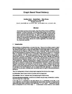
Figure 1: Example of saliency map generation where the proposed system (SalGAN) outperforms a standard binary cross entropy (BCE) prediction model.
capture the human attention. These saliency maps have been used as soft-attention guides for other computer vision tasks, and also directly for user studies in fields like marketing. This paper introduces the usage of generative adversarial networks (GANs)[7] for visual saliency prediction. In this context, training is driven by two agents. First, the generator that creates a synthetic sample matching the data distribution modelled by a training data set; second, the discriminator, that distinguishes between a real sample drawn directly from the training data set and one created by the generator. In our case, this data distribution corresponds to pairs of real images and their corresponding visual saliency maps. The generator, named in our work SalGAN, is the only responsible for generating the saliency map for a given image and uses a deep convolutional neural network (DCNN) to produce such maps. This network is initially trained with a binary cross entropy (BCE) loss over downsampled versions
1. Motivation Visual saliency prediction in computer vision aims at estimating the locations in an image that attract the attention of humans. Salient points in an image are understood as a result of a bottom-up process where a human observer explores the image for a few seconds with no particular task in mind. These data are traditionally measured with eye-trackers, and more recently with mouse clicks [12] or webcams [15]. The salient points over the image are usually aggregated and represented in a saliency map, a single channel image obtained by convolving each point with a Gaussian kernel. As a result, a gray-scale image or heatmap is generated to represent the probability of each corresponding pixel in the image to 1
of the saliency maps. The model is refined with a discriminator network trained to solve a binary classification task between the saliency maps generated by SalGAN and the real ones used as ground truth. Our experiments show how adversarial training allows reaching state-of-the-art performance across different metrics when combined with a BCE content loss in a single-tower and single-task model. The amount of different metrics to evaluate visual saliency prediction is broad and diverse, and the discussion about them is rich and active. Pioneering metrics have saturated with the introduction of deep learning models trained on large data sets, boosting the proposal of new metrics and challenges for the community. The widely adopted MIT300 benchmark evaluates its results on 8 different metrics, and the more recent LSUN challenge on the SALICON data set considers four of them. Also recently, the Information Gain (IG) value has been presented as powerful relative metric in the field. The diversity of metrics in our current deep learning era has resulted also in a diversity of loss functions between state-of-the-art solutions. Models based on backpropagation training have adopted loss functions capable to capture the different features assessed by the multiple metrics. Our approach, though, differs from other state-ofthe-art solutions as we focus on exploring the benefits of introducing the agnostic loss function proposed in generative adversarial training. This paper explores adversarial training for visual saliency prediction, showing how the simple binary classification between real and synthetic samples significantly benefits a wide range of visual saliency metrics, without needing to specify a tailored loss function. Our results achieve state-of-the-art performance with a simple DCNN whose parameters are refined with a discriminator. As a secondary contribution, we show the benefits of using the binary cross entropy (BCE) loss function and downsampled saliency maps when training this DCNN. The remaining of the work is organized as follows. Section 2 reviews the state-of-the-art models for visual saliency prediction, discussing the loss functions they are based upon, their relations with the different metrics as well as their complexity in terms of architecture and training. Section 3 presents SalGAN, our deep convolutional neural network based on a convolutional encoder-decoder architecture, as well as the discriminator network used during its adversarial training. Section 4 describes the training process of SalGAN and the loss functions used. Section 5 includes the experiments and results of the presented techniques. Finally, Section 6 closes the paper by drawing the main conclusions.
low-level features at multiple scales and combining them to form a saliency map. Harel et al. [8], also starting from low-level feature maps, introduced a graph-based saliency model that defines Markov chains over various image maps, and treat the equilibrium distribution over map locations as activation and saliency values. Judd et al. in [14] presented a bottom-up, top-down model of saliency based not only on low but mid and high-level image features. Borji [1] combined low-level features saliency maps of previous best bottom-up models with top-down cognitive visual features and learned a direct mapping from those features to eye fixations. As in many other fields in computer vision, a number of deep learning solutions have very recently been proposed that significantly improve performance. For example, as stated in [4], among the top 10 results in the MIT saliency benchmark [2], as of March 2016, six models were based on deep learning. When considering AUC-Judd as the reference metric, results as of September 2016 on the MIT300 benchmark include only one non-deep learning technique (Boolean map saliency [31]) among the top-ten. The Ensemble of Deep Networks (eDN) [30] represented an early architecture that automatically learns the representations for saliency prediction, blending feature maps from different layers. Their network might be consider a shallow network given the number of layers. In [25] shallow and deeper networks were compared. DCNN have shown better results even when pre-trained with datasets build for other purposes. DeepGaze [19] provided a deeper network using the well-know AlexNet [16], with pre-trained weights on Imagenet [6] and with a readout network on top whose inputs consisted of some layer outputs of AlexNet. The output of the network is blurred, center biased and converted to a probability distribution using a softmax. A new version called DeepGaze 2 [21] using VGG-19 [27] and trained with the SALICON dataset [12] has recently achieved the best results in the MIT saliency benchmark. Kruthiventi et al. [18] also used pre-trained VGG networks and the SALICON dataset to obtain saliency prediction maps with outstanding results. This network uses additional inception modules [28] to model fine and coarse saliency details. Huang et al. [9], in the so call SALICON net, obtained better results by using VGG rather than AlexNet or GoogleNet [28]. In their proposal they considered two networks with fine and coarse inputs, whose feature maps outputs are concatenated. Following this idea of modeling local and global saliency features, Liu et al. [22] proposed a multiresolution convolutional neural network that is trained from image regions centered on fixation and non-fixation locations over multiple resolutions. Diverse top-down visual features can be learned in higher layers and bottom-up visual saliency can also be inferred by combining information over multiple resolutions. These ideas are further developed in they recent work called
2. Related work Saliency prediction has received interest by the research community for many years. Thus seminal works by Itti et al. [10] proposed to predict saliency maps considering 2
Image Stimuli + Predicted Saliency Map Generator
Discriminator
BCE Cost
Conv-VGG Conv-Scratch
Max Pooling Fully Connected
Upsampling
Adversarial Cost
Sigmoid
Image Stimuli + Ground Truth Saliency Map
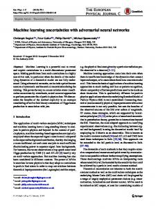
Figure 2: Overall architecture of the proposed saliency map estimation system. In our work we present a network architecture that takes a different approach and we consider loss functions that are well adapted to our model. In particular other proposals use losses based on MSE or similar [5], [25], [17], whereas we use BCE and compare it with MSE as a reference.
DSCLRCN [24], where the proposed model learns saliency related local features on each image location in parallel and then learns to simultaneously incorporate global context and scene context to infer saliency. They incorporate a model to effectively learn long-term spatial interactions and scene contextual modulation to infer image saliency. Their experiments have obtained outstanding results in the MIT Saliency Benchmark. Cornia et al. [5] proposed an architecture that combines features extracted at different levels of a DCNN. Their model is composed of three main blocks: a feature extraction DCNN, a feature encoding network, which weights low and high-level feature maps, and a prior learning network. They also introduce a loss function inspired by three objectives: to measure similarity with the ground truth, to keep invariance of predictive maps to their maximum and to give importance to pixels with high ground truth fixation probability. In fact choosing an appropriate loss function has become an issue that can lead to improved results. Thus, another interesting contribution of Huang et al. [9] lies on minimizing loss functions based on metrics that are differentiable, such as NSS, CC, SIM and KL divergence to train the network (see [26] and [20] for the definition of these metrics. A thorough comparison of metrics can be found in [3]). In Huang’s work [9] KL divergence gave the best results. Jetley et al. [11] also tested loss functions based on probability distances, such as X2 divergence, total variation distance, KL divergence and Bhattacharyya distance by considering saliency map models as generalized Bernoulli distributions. The Bhattacharyya distance was found to give the best results. Finally, the work by Johnson et al. [13] defines a perceptual loss combining a per-pixel loss together with another loss term based on the semantics of the image. It is applied to image style transfer but it may be used in models for saliency prediction.
3. Architecture The architecture of the presented SalGAN is based on two deep convolutional neural network (DCNN) modules, namely the generator and discriminator, whose combined efforts aim at predicting a visual saliency map for a given input image. This section provides details on the structure of both modules, the considered loss functions, and the initialization before beginning adversarial training.
3.1. Generator SalGAN follows a convolutional encoder-decoder architecture, where the encoder part includes max pooling layers that decrease the size of the feature maps, while the decoder part uses upsampling layers followed by convolutional filters to construct an output that is the same resolution as the input. Figure 2 shows the architecture of the system. The encoder part of the network is identical in architecture to VGG-16 [27], omitting the final pooling and fully connected layers. The network is initialized with the weights of a VGG-16 model trained on the ImageNet data set for object classification [6]. Only the last two groups of convolutional layers in VGG-16 are modified during the training for saliency prediction, while the earlier layers remain fixed from the original VGG-16 model. We fix weights to save computational resources during training, even at the possible expense of some loss in performance.
3
layer
depth
kernel
stride
pad
activation
conv1 1 conv1 2 pool1
3 32
1×1 3×3 2×2
1 1 2
1 1 0
ReLU ReLU -
conv2 1 conv2 2 pool2
64 64
3×3 3×3 2×2
1 1 2
1 1 0
ReLU ReLU -
conv3 1 conv3 2 pool3
64 64
3×3 3×3 2×2
1 1 2
1 1 0
ReLU ReLU -
100 2 1
-
-
-
tanh tanh sigmoid
fc4 fc5 fc6
ˆ is defined between the predicted saliency function L(S, S) ˆ map S and its corresponding ground truth S. The first considered content loss is mean squared error (MSE) or Euclidean loss, defined as: LM SE =
N 1 X (Sj − Sˆj )2 . N j=1
(1)
In our work, MSE is used as a baseline reference, as it has been adopted directly or with some variations in other state of the art solutions for visual saliency prediction [25, 17, 5]. Solutions based on MSE aim at maximizing the peak signal-to-noise ratio (PSNR). These works tend to filter high spatial frequencies in the output, favoring this way blurred contours. MSE corresponds to computing the Euclidean distance between the predicted saliency and the ground truth. Ground truth saliency maps are normalized so that each value is in the range [0, 1]. Saliency values can therefore be interpreted as estimates of the probability that a particular pixel is attended by an observer. It is tempting to therefore induce a multinomial distribution on the predictions using a softmax on the final layer. Clearly, however, more than a single pixel may be attended, making it more appropriate to treat each predicted value as independent of the others. We therefore propose to apply an element-wise sigmoid to each output in the final layer so that the pixel-wise predictions can be thought of as probabilities for independent binary random variables. An appropriate loss in such a setting is the binary cross entropy, which is the average of the individual binary cross entropies (BCE) across all pixels:
Table 1: Architecture of the discriminator network.
The decoder architecture is structured in the same way as the encoder, but with the ordering of layers reversed, and with pooling layers being replaced by upsampling layers. Again, ReLU non-linearities are used in all convolution layers, and a final 1 × 1 convolution layer with sigmoid nonlinearity is added to produce the saliency map. The weights for the decoder are randomly initialized.
3.2. Discriminator Table 1 gives the architecture and layer configuration for the discriminator. In short, the network is composed of six 3x3 kernel convolutions interspersed with three pooling layers (↓2), and followed by three fully connected layers. The convolution layers all use ReLU activations while the fully connected layers employ tanh activations, with the exception of the final layer, which uses a sigmoid activation.
LBCE = −
N 1 X Sj log(Sˆj ) + (1 − Sj ) log(1 − Sˆj ). N j=1
(2)
4.2. Adversarial loss
4. Training
Generative adversarial networks (GANs) [7] are commonly used to generate images with realistic statistical properties. The idea is to simultaneously fit two parametric functions. The first of these functions, known as the generator, is trained to transform samples from a simple distribution (e.g. Gaussian) into samples from a more complicated distribution (e.g. natural images). The second function, the discriminator, is trained to distinguish between samples from the true distribution and generated samples. Training proceeds alternating between training the discriminator using generated and real samples, and training the generator, by keeping the discriminator weights constant and backpropagating the error through the discriminator to update the generator weights. The saliency prediction problem has some important differences from the above scenario. First, the objective is to fit a deterministic function that generates realistic saliency
The filter weights in SalGAN have been trained over a perceptual loss [13] resulting from combining a content and adversarial loss. The content loss follows a classic approach in which the predicted saliency map is pixel-wise compared with the corresponding one from ground truth. The adversarial loss depends of the real/synthetic prediction of the discriminator over the generated saliency map.
4.1. Content loss The content loss is computed in a per-pixel basis, where each value of the predicted saliency map is compared with its corresponding peer from the ground truth map. Given an image I of dimensions N = W × H, we represent the saliency map S as vector of probabilities where Sj ∈ RN is the probability of pixel Ij being fixated. A content loss 4
values from images, rather than realistic images from random noise. As such, in our case the input to the generator is not random noise but an image. Second, it is clear that knowledge of the image that a saliency map corresponds to to is essential to evaluate quality. We therefore include both the image and saliency map as inputs to the discriminator. Finally, when using generative adversarial networks to generate realistic images, there is generally no ground truth to compare against. In our case, however, the corresponding ground truth saliency map is available. When updating the parameters of the generator function, we found that using a loss function that is a combination of the error from the discriminator and the cross entropy with respect to the ground truth improved the stability and convergence rate of the adversarial training. The final loss function for the generator during adversarial training can be formulated as: ˆ LGAN = α· LBCE − log D(I, S),
BCE BCE/2 BCE/4 BCE/8
sAUC ↑
AUC-B ↑
NSS ↑
CC ↑
IG ↑
0.752 0.750 0.755 0.754
0.825 0.820 0.831 0.827
2.473 2.527 2.511 2.503
0.761 0.764 0.763 0.762
0.712 0.592 0.825 0.831
Table 2: Impact of downsampled saliency maps at (15 epochs) evaluated over SALICON validation. BCE/x refers to a downsample factor of 1/x over a saliency map of 256 × 192. for SalGAN were run using the train and validation partitions of the SALICON dataset [12]. This is a large dataset built by collecting mouse clicks on a total of 20,000 images from the Microsoft Common Objects in Context (MSCoCo) dataset [23]. We have adopted this dataset for our experiments because it is the largest one available for visual saliency prediction. In addition to SALICON, Section 5.3 also presents results on MIT300, the benchmark with the largest amount of submissions.
(3)
ˆ is the probability of fooling the discriminator, where D(I, S) so that the loss associated to the generator will grow more when chances of fooling the discriminator are lower. In our experiments, we used an hyperparameter of α = 0.05. During the training of the discriminator, no content loss is available and the sign of the adversarial term is switched. At train time, we first bootstrap the generator function by training for 15 epochs using only BCE, which is computed with respect to the downsampled output and ground truth saliency. After this, we add the discriminator and begin adversarial training. The input to the discriminator network is an RGBS image of size 256 × 192 × 4 containing both the source image channels and (predicted or ground truth) saliency. We train the networks on the 10,000 images from the SALICON training set using a batch size of 32. This was the largest batch size we could use given the memory constraints of our hardware. During the adversarial training, we alternate the training of the generator and discriminator after each iteration (batch). We used L2 weight regularization (i.e. weight decay) when training both the generator and discriminator (λ = 1 × 10⁻⁴ ). We used AdaGrad for optimization, with an initial learning rate of 3 × 10⁻⁴ .
5.1. Non-adversarial training The two content losses presented in Section 4.1, MSE and BCE, were compared to define a baseline upon which we later assess the impact of the adversarial training. The two first rows of Table 3 shows how a simple change from MSE to BCE brings a consistent improvement in all metrics. This improvement suggests that treating saliency prediction as multiple binary classification problem is more appropriate than treating it as a standard regression problem, in spite of the fact that the target values are not binary. Minimizing cross entropy is equivalent to minimizing the KL divergence between the predicted and target distributions, which is a reasonable objective if both predictions an targets are interpreted as probabilities. Based on the superior BCE-based loss compared with MSE, we also explored the impact of computing the content loss over downsampled versions of the saliency map. This technique reduces the required computational resources at both training and test times and, as shown in Table 2, not only does it not decrease performance, but it can actually improve it. Given this results, we chose to train SalGAN on saliency maps downsampled by a factor 1/4, which in our architecture corresponds to saliency maps of 64 × 48.
5. Experiments The presented SalGAN model for visual saliency prediction was assessed and compared from different perspectives. First, the impact of using BCE and the downsampled saliency maps are assessed. Second, the gain of the adversarial loss is measured and discussed, both from a quantitative and a qualitative point of view. Finally, the performance of SalGAN is compared to both published and unpublished works to compare its performance with the current state-of-the-art. The experiments aimed at finding the best configuration
5.2. Adversarial gain The gain achieved by introducing the adversarial loss into the perceptual loss (see Section 4.2) was assessed by using BCE as a content loss and feature maps of 68 × 48. The first row of results in Table 3 refers to a baseline defined by training SalGAN with the BCE content loss for 15 epochs 5
AUC Judd
Sim
0.665 0.660 20
40
60
0.876 20
0.840 0.830
CC
AUC Borji
GAN+BCE BCE Only
0.878
80 100 120
0.850
0.820 0.810 40
60
80 100 120
IG (Gaussian)
20
NSS
0.880
0.874
0.655
2.600 2.580 2.560 2.540 2.520 2.500 2.480 2.460 2.440
sAUC ↑
AUC-B ↑
NSS ↑
CC ↑
IG
MSE BCE
0.728 0.753
0.820 0.825
1.680 2.562
0.708 0.772
0.628 0.824
BCE/4 GAN/4
0.757 0.773
0.833 0.859
2.580 2.589
0.772 0.786
1.067 1.243
0.882
0.670
20
40
60
80 100 120
epoch
0.790 0.785 0.780 0.775 0.770 0.765 0.760 0.755
20
40
40
60
60
80 100 120
Table 3: Best results through epochs obtained with nonadversarial (MSE and BCE) and adversarial (GAN) training. BCE/4 and GAN/4 refer to downsampled saliency maps. Saliency maps assessed on SALICON validation.
80 100 120
1.100 1.000
5.3. Comparison with the state-of-the-art
0.900
SalGAN is compared in Table 4 to several other algorithms from the state-of-the-art. The comparison is based on the evaluations run by the organizers of the SALICON and MIT300 benchmarks on a test dataset whose ground truth is not public. The two benchmarks offer complementary features: while SALICON is a much larger dataset with 5,000 test images, MIT300 has attracted the participation of many more researchers. In both cases, SalGAN was trained using 15,000 images contained in the training (10,000) and validation (5,000) partitions of the SALICON dataset. Notice that while both datasets aim at capturing visual saliency, the acquising of data differed, as SALICON ground truth was generated based on crowdsourced mouse clicks, while the MIT300 was built with eye trackers on a limited and controlled group of users. Table 4 compares SalGAN not only with published models, but also with works that have not been peer reviewed. SalGAN presents very competitive results in both datasets, as it improves or equals the performance of all other models in at least one metric.
0.800 0.700
20
40
60
80 100 120
epoch
Figure 3: SALICON validation set accuracy metrics for GAN+BCE vs BCE on varying numbers of epochs. AUC shuffled is omitted as the trend is identical to that of AUC Judd. only. Later, two options are considered: 1) training based on BCE only (2nd row), or 2) introducing the adversarial loss (3rd and 4th row). Figure 3 compares validation set accuracy metrics for training with combined GAN and BCE loss versus a BCE alone as the number of epochs increases. In the case of the AUC metrics (Judd and Borji), increasing the number of epochs does not lead to significant improvements when using BCE alone. The combined BCE/GAN loss however, continues to improve performance with further training. After 100 and 120 epochs, the combined GAN/BCE loss shows substantial improvements over BCE for five of six metrics. The single metric for which GAN training fails to improve performance is normalized scanpath saliency (NSS). The reason for this may be that GAN training tends to produce a smoother and more spread out estimate of saliency, which better matches the statistical properties of real saliency maps, but may increase the false positive rate. As noted by Bylinskii et al. [3], NSS is very sensitive to such false positives. The impact of increased false positives depends on the final application. In applications where the saliency map is used as a multiplicative attention model (e.g. in retrieval applications, where spatial features are importance weighted), false positives are often less important than false negatives, since while the former includes more distractors, the latter removes potentially useful features. Note also that NSS is differentiable, so could potentially be optimized directly when important for a particular application.
5.4. Qualitative results The impact of adversarial training has also been explored from a qualitative perspective by observing the resulting saliency maps. Figure 4 shows three examples from the MIT300 dataset, highlighted by Bylinskii et al. [4] as being particular challenges for existing saliency algorithms. The areas highlighted in yellow in the images on the left are regions that are typically missed by algorithms. In the first example, we see that SalGAN successfully detects the often missed hand of the magician and face of the boy as being salient. The second example illustrates a failure case where SalGAN, like other algorithms, also fails to place sufficient saliency on the area around the white ball (though this region does have more saliency than most of the rest of the image). The final example illustrates what we believe to be one of the limitations of this dataset. The ground truth places most of the saliency on the smaller text at the bottom of the sign. This is because observers tend spend more time attending 6
SALICON (test)
AUC-J ↑
Sim ↑
EMD ↓
AUC-B ↑
sAUC ↑
CC ↑
NSS ↑
KL ↓
DSCLRCN [24](*) SalGAN ML-NET [5] SalNet [25] MIT300
AUC-J ↑
Sim ↑
EMD ↓
0.884 0.884 (0.866) (0.858) AUC-B ↑
0.776 0.772 (0.768) (0.724) sAUC ↑
0.831 0.781 (0.743) (0.609) CC ↑
3.157 2.459 2.789 (1.859) NSS ↑
KL ↓
0.92 0.88 0.87 0.87 0.87 0.86 (0.85) (0.85) (0.84) (0.84) (0.83) (0.83)
1.00 (0.46) 0.68 0.67 (0.60) 0.63 (0.60) (0.59) (0.39) (0.57) (0.52) (0.51)
0.00 (3.98) 2.17 2.04 (2.62) 2.29 (2.58) (2.63) (4.97) (2.72) (3.31) (3.35)
0.88 0.86 (0.79) (0.80) 0.85 0.81 (0.80) (0.75) 0.83 0.81 0.82 0.82
0.81 0.72 0.72 (0.71) 0.74 0.72 0.73 (0.70) (0.66) (0.68) (0.69) (0.65)
1.0 (0.52) 0.80 0.78 0.74 0.73 (0.70) (0.67) (0.48) (0.65) (0.58) (0.55)
3.29 (1.29) 2.35 2.26 2.12 2.04 2.05 2.05 (1.22) (1.78) (1.51) (1.41)
0.00 (0.96) 0.95 0.63 0.54 1.07 0.92 (1.10) (1.23) 0.65 0.81 0.81
Humans Deep Gaze II [21](*) DSCLRCN [24](*) DeepFix [17](*) SALICON [9] SalGAN PDP [11] ML-NET [5] Deep Gaze I [19] iSEEL [29](*) SalNet [25] BMS [31]
Table 4: Comparison of SalGAN with other state-of-the-art solutions on the SALICON (test) and MIT300 benchmarks according to their public leaderboards on November 10, 2016. Values in brackets correspond to performances worse than SalGAN. (*) indicates citations to non-peer reviewed texts. this area (reading the text), and not because it is the first area that observers tend to attend. Existing metrics, however, tend to be agnostic to the order in which areas are attended, a limitation we hope to look into in the future. Figure 5 illustrates the effect of adversarial training on the statistical properties of the generated saliency maps. Shown are two close up sections of a saliency map from cross entropy training (left) and adversarial training (right). Training on BCE alone produces saliency maps that while they may be locally consistent with the ground truth, are often less smooth and have complex level sets. GAN training on the other hand produces much smoother and simpler level sets. Finally, Figure 6 shows some qualitative results comparing the results from training with MSE, BCE, and BCE/GAN against the ground truth for images from the SALICON validation set.
It is worth pointing out that although we use a VGG-16 based encoder-decoder model as the generator in this paper, the proposed GAN training approach is generic and could be applied to improve the performance of other deep saliency models. For example, the authors of the DSCLRCN model observed that ResNet-based architectures outperformed VGG-based ones for saliency prediction, and that using multiple image scales improves accuracy. Similar modifications to our model would likely provide similar gains. Further improvements could also likely be achieved by carefully tuning hyperparameters, and in particular the tradeoff between BCE and GAN loss in Equation 3, which we did not attempt to optimize for this paper. Finally, an ensemble of models is also likely to improve performance, at the cost of additional computation at predict time. Our results can be reproduced with the source code and trained models available at https://imatge-upc. github.io/saliency-salgan-2017/.
6. Conclusions In this work we have shown how adversarial training over a deep convolutional neural network can achieve state-of-theart performance with a simple encoder-decoder architecture. A BCE-based content loss was shown to be effective for both initializing the generator, and as a regularization term for stabilizing adversarial training. Our experiments showed that adversarial training improved all bar one saliency metric when compared to further training on cross entropy alone.
7. Acknowledgments The Image Processing Group at UPC is supported by the project TEC2013-43935-R and TEC2016-75976-R, funded by the Spanish Ministerio de Economia y Competitividad and the European Regional Development Fund (ERDF). The Image Processing Group at UPC is a SGR14 Consolidated Research Group recognized and sponsored by the Catalan Government (Generalitat de Catalunya) through its AGAUR 7
Images
Ground Truth
MSE
BCE
SalGAN
Figure 6: Qualitative results of SalGAN on the SALICON validation set.
References
office. The contribution from the Barcelona Supercomputing Center has been supported by project TIN2015-65316 by the Spanish Ministry of Science and Innovation contracts 2014SGR-1051 by Generalitat de Catalunya. This material is based upon works supported by Science Foundation Ireland under Grant No 15/SIRG/3283. We gratefully acknowledge the support of NVIDIA Corporation with the donation of a GeForce GTX Titan Z used in this work, together with the support of BSC/UPC NVIDIA GPU Center of Excellence. We also want to thank all the members of the X-theses group for their advice, especially to Victor Garcia and Santi Pascual for their proof reading.
[1] A. Borji. Boosting bottom-up and top-down visual features for saliency estimation. In IEEE Conference on Computer Vision and Pattern Recognition (CVPR), 2012. [2] Z. Bylinskii, T. Judd, A. Ali Borji, L. Itti, F. Durand, A. Oliva, and A. Torralba. MIT saliency benchmark. http://saliency.mit.edu/. [3] Z. Bylinskii, T. Judd, A. Oliva, A. Torralba, and F. Durand. What do different evaluation metrics tell us about saliency models? ArXiv preprint:1610.01563, 2016. [4] Z. Bylinskii, A. Recasens, A. Borji, A. Oliva, A. Torralba, and F. Durand. Where should saliency models look next? In European Conference on Computer Vision (ECCV), 2016. [5] M. Cornia, L. Baraldi, G. Serra, and R. Cucchiara. A deep multi-level network for saliency prediction. In International
8
Ground truth
SalGAN [10]
[11]
[12]
[13]
[14]
[15]
[16]
Figure 4: Example images from MIT300 containing salient region (marked in yellow) that is often missed by computational models, and saliency map estimated by SalGAN.
[17]
[18]
[19]
Figure 5: Close-up comparison of output from training on BCE loss vs combined BCE/GAN loss. Left: saliency map from network trained with BCE loss. Right: saliency map from proposed GAN training.
[20]
[21] Conference on Pattern Recognition (ICPR), 2016. [6] J. Deng, W. Dong, R. Socher, L.-J. Li, K. Li, and L. Fei-Fei. ImageNet: A large-scale hierarchical image database. In IEEE Conference on Computer Vision and Pattern Recognition (CVPR), 2009. [7] I. Goodfellow, J. Pouget-Abadie, M. Mirza, B. Xu, D. WardeFarley, S. Ozair, A. Courville, and Y. Bengio. Generative adversarial nets. In Advances in Neural Information Processing Systems, pages 2672–2680, 2014. [8] J. Harel, C. Koch, and P. Perona. Graph-based visual saliency. In Neural Information Processing Systems (NIPS), 2006. [9] X. Huang, C. Shen, X. Boix, and Q. Zhao. Salicon: Reducing the semantic gap in saliency prediction by adapting deep neu-
[22]
[23]
[24]
[25]
9
ral networks. In IEEE International Conference on Computer Vision (ICCV), 2015. L. Itti, C. Koch, and E. Niebur. A model of saliency-based visual attention for rapid scene analysis. IEEE Transactions on Pattern Analysis and Machine Intelligence (PAMI), (20):1254– 1259, 1998. S. Jetley, N. Murray, and E. Vig. End-to-end saliency mapping via probability distribution prediction. In IEEE Conference on Computer Vision and Pattern Recognition (CVPR), 2016. M. Jiang, S. Huang, J. Duan, and Q. Zhao. Salicon: Saliency in context. In IEEE Conference on Computer Vision and Pattern Recognition (CVPR), 2015. J. Johnson, A. Alahi, and L. Fei-Fei. Perceptual losses for real-time style transfer and super-resolution. In European Conference on Computer Vision (ECCV), 2016. T. Judd, K. Ehinger, F. Durand, and A. Torralba. Learning to predict where humans look. In IEEE International Conference on Computer Vision (ICCV), 2009. K. Krafka, A. Khosla, P. Kellnhofer, H. Kannan, S. Bhandarkar, W. Matusik, and A. Torralba. Eye tracking for everyone. In IEEE Conference on Computer Vision and Pattern Recognition (CVPR), 2016. A. Krizhevsky, I. Sutskever, and G. E. Hinton. ImageNet classification with deep convolutional neural networks. In Advances in neural information processing systems, pages 1097–1105, 2012. S. S. Kruthiventi, K. Ayush, and R. V. Babu. Deepfix: A fully convolutional neural network for predicting human eye fixations. ArXiv preprint:1510.02927, 2015. S. S. Kruthiventi, V. Gudisa, J. Dholakiya, and R. V. Babu. Saliency unified: A deep architecture for simultaneous eye fixation prediction and salient object segmentation. In IEEE Conference on Computer Vision and Pattern Recognition (CVPR), 2016. M. K¨ummerer, L. Theis, and M. Bethge. DeepGaze I: Boosting saliency prediction with feature maps trained on ImageNet. In International Conference on Learning Representations (ICLR), 2015. M. K¨ummerer, L. Theis, and M. Bethge. Informationtheoretic model comparison unifies saliency metrics. Proceedings of the National Academy of Sciences (PNAS), 112(52):16054–16059, 2015. M. K¨ummerer, T. S. Wallis, and M. Bethge. DeepGaze II: Reading fixations from deep features trained on object recognition. ArXiv preprint:1610.01563, 2016. G. Li and Y. Yu. Visual saliency based on multiscale deep features. In IEEE Conference on Computer Vision and Pattern Recognition (CVPR), 2015. T.-Y. Lin, M. Maire, S. Belongie, J. Hays, P. Perona, D. Ramanan, P. Doll´ar, and L. Zitnick. Microsoft COCO: Common objects in context. In European Conference on Computer Vision (ECCV), 2014. N. Liu and J. Han. A deep spatial contextual long-term recurrent convolutional network for saliency detection. ArXiv preprint:1610.01708, 2016. J. Pan, E. Sayrol, X. Gir´o-i Nieto, K. McGuinness, and N. E. O’Connor. Shallow and deep convolutional networks for
[26]
[27]
[28]
[29]
[30]
[31]
saliency prediction. In IEEE Conference on Computer Vision and Pattern Recognition (CVPR), 2016. N. Riche, D. M., M. Mancas, B. Gosselin, and T. Dutoit. Saliency and human fixations. state-of-the-art and study comparison metrics. In IEEE International Conference on Computer Vision (ICCV), 2013. K. Simonyan and A. Zisserman. Very deep convolutional networks for large-scale image recognition. In International Conference on Learning Representations (ICLR), 2015. C. Szegedy, W. Liu, Y. Jia, P. R. S. Sermanet, D. Anguelov, D. Erhan, V. Vanhoucke, and A. Rabinovich. Going deeper with convolutions. In IEEE Conference on Computer Vision and Pattern Recognition (CVPR), 2015. H. R. Tavakoli, A. Borji, J. Laaksonen, and E. Rahtu. Exploiting inter-image similarity and ensemble of extreme learners for fixation prediction using deep features. ArXiv preprint:1610.06449, 2016. E. Vig, M. Dorr, and D. Cox. Large-scale optimization of hierarchical features for saliency prediction in natural images. In IEEE Conference on Computer Vision and Pattern Recognition (CVPR), 2014. J. Zhang and S. Sclaroff. Saliency detection: a boolean map approach. In IEEE International Conference on Computer Vision (ICCV), 2013.
10


![NIPS 2016 Tutorial: Generative Adversarial Networks - arXiv [PDF]](https://m.moam.info/img/260x300/nips-2016-tutorial-generative-adversarial-networks_649b8ca7098a9ec8508b45c4.jpg)