Feb 10, 2015 - Spectral Densities (PSD) of the sources are available; these are commonly called spectrograms .... Examples of kernels to use for KAM in audio (from [17]). The waveforms are then .... webpage of this paper1. IV. EVALUATION.
Scalable audio separation with light kernel additive modelling Antoine Liutkus, Derry Fitzgerald, Zafar Rafii
To cite this version: Antoine Liutkus, Derry Fitzgerald, Zafar Rafii. Scalable audio separation with light kernel additive modelling. IEEE International Conference on Acoustics, Speech and Signal Processing (ICASSP) , Apr 2015, Brisbane, Australia. 2015.
HAL Id: hal-01114890 https://hal.inria.fr/hal-01114890v2 Submitted on 10 Feb 2015
HAL is a multi-disciplinary open access archive for the deposit and dissemination of scientific research documents, whether they are published or not. The documents may come from teaching and research institutions in France or abroad, or from public or private research centers.
L’archive ouverte pluridisciplinaire HAL, est destin´ee au d´epˆot et `a la diffusion de documents scientifiques de niveau recherche, publi´es ou non, ´emanant des ´etablissements d’enseignement et de recherche fran¸cais ou ´etrangers, des laboratoires publics ou priv´es.
SCALABLE AUDIO SEPARATION WITH LIGHT KERNEL ADDITIVE MODELLING Antoine Liutkus1
Derry Fitzgerald2
Zafar Rafii3
1
Inria, speech processing team, Villers-lès-Nancy, France NIMBUS Centre, Cork Institute of Technology, Ireland 3 Gracenote, Media Technology Lab, Emeryville, CA, USA 2
ABSTRACT Recently, Kernel Additive Modelling (KAM) was proposed as a unified framework to achieve multichannel audio source separation. Its main feature is to use kernel models for locally describing the spectrograms of the sources. Such kernels can capture source features such as repetitivity, stability over time and/or frequency, self-similarity, etc. KAM notably subsumes many popular and effective methods from the state of the art, including REPET and harmonic/percussive separation with median filters. However, it also comes with an important drawback in its initial form: its memory usage badly scales with the number of sources. Indeed, KAM requires the storage of the full-resolution spectrogram for each source, which may become prohibitive for full-length tracks or many sources. In this paper, we show how it can be combined with a fast compression algorithm of its parameters to address the scalability issue, thus enabling its use on small platforms or mobile devices. Index Terms—sound source separation, Kernel Additive Modelling, randomized algorithms I. INTRODUCTION Musical audio source separation aims at recovering the constituent isolated instrumental stems from a musical track. It is a topic that has many applications in the entertainment industry such as automatic karaoke [19], [29], music upmixing [21], [22], [23] or audio restoration [31]. For this reason, it has gathered the attention of a large community of researchers in the past 15 years [35], [34]. The inherent difficulty of audio source separation comes from the fact that it is essentially an ill-posed inverse problem: in a typical setting, we have more signals to estimate than the number of signals we observe. Indeed, music most often comes in mono or stereo recordings, while our objective is to recover all its constituent instrumental sources, with there being typically 5 to 10 sources. Hence, we have more unknowns than available equations to describe the complex mixing process we want to invert. Without any further regularization scheme, there is an infinite number of solutions to this so-called underdetermined problem. In order to perform audio source separation, all techniques therefore include some kind of knowledge in the modelling in order to restrict the search for solutions. This enforces the fact that neither the mixing process nor the source signals should be completely arbitrary. In the overdetermined case, i.e. when there are more mixtures than sources, only a linear mixing model and very loose probabilistic assumptions on the sources signals were shown necessary for building a time-invariant demixing filter, as demonstrated by the popular Independent Components Analysis (ICA, see e.g. [14]) or Second-Order Blind Identification (SOBI [1]) approaches (see [5] for an overview). On the contrary, it is not possible to design such a time-invariant demixing filter in the underdetermined case: only time-varying adaptive processing permits separation of sources. Many approaches were explored for this purpose, including statespace modelling [4], sparse decompositions [27] and, finally, local Gaussian modelling (LGM, [6], [26], [15]). In this latter model, it
has been showed that very good separation can be obtained through generalized Wiener filtering, provided good estimates for the Power Spectral Densities (PSD) of the sources are available; these are commonly called spectrograms in the literature. While blind underdetermined separation can be achieved under the LGM by exploiting only spatial (multichannel) information [6], experience shows that further constraining the sources PSD models yields much better results in practice. This track of research increasingly showed that prior assumptions about the sources leads to improved performance in practice [33], [16], [34]. The common ground of most related work on audio source separation then becomes the building of models for the spectrograms of the sources that have a strong expressive power while requiring the fitting of only a small number of parameters. On this topic, we can identify two main directions in recent research. First, instead of assuming the PSD of a source to be completely arbitrary, as done in [6], we can suppose that it exhibits some kind of known structure through the use of a global parametric model. A popular choice for this purpose is to express the spectrogram of a source as the activation over time of only a few spectral patterns. This idea leads to the celebrated Nonnegative Matrix Factorization framework (NMF, [32], [24], [7], [26], [15]). Second, even if NMF often yields good performance, it is limited in the sense that some sources cannot be well described as the superposition of only a few spectral templates. Rather, there are cases where it is more convenient to impose only some kind of local regularities on the spectrograms of the sources to identify them from the mixture instead of a global and much constrained model. For instance, if we know that a musical background is repetitive whereas the vocal signal is not, it is much more efficient to enforce this knowledge rather than to choose a NMF model. This line of thought leads to the REPET algorithm [28], [19], [29], that proved very efficient for music/voice separation. Likewise, if our objective is to separate harmonic and percussive sounds, there is no real advantage in trying to build dictionaries of such sounds to use for NMF as in [15]. On the contrary, experience shows that it is much more effective to directly exploit the fact that harmonic spectrograms should be locally constant along time while percussive spectrograms are locally constant along frequency. Enforcing this knowledge is very easily done through simple median filters as in [9]. More generally, we recently showed that all those techniques may be seen as particular cases of a general framework called Kernel Additive Modelling (KAM, [17]), where the spectrogram of each source is modelled only locally. We showed in [17], [20] that the resulting iterative Kernel Back-Fitting audio separation algorithm (KBF) basically amounts to median-filtering the spectrogram of each source estimate at each iteration. The kernel used for this median filter depends on the source and encodes our prior knowledge about it. This approach generalizes many state of the art techniques and was shown to give good results for different audio separation tasks such as voice/music separation [20] or harmonic/percussive separation [11]. Although it gives a very satisfying performance in many cases,
the KAM framework comes with an important drawback, which is memory usage: it requires storing the full spectrogram of each source. Indeed, since the assumptions about a source spectrogram in KAM are only described in terms of local constraints: it does not automatically come with a concise model as NMF modelling does. Hence, if we are to separate 10 sources, say, from a 4 minutes song, we need to store the equivalent of 40 minutes of audio at full resolution in a highly redundant representation, in practice requiring approximately 32GB of RAM in our implementations [17], [20]. This prevents the method being used on today’s standard laptop computers or mobile devices, in sharp contrast with NMF-based methods whose memory usage is much smaller. In this paper, we address this memory usage issue of KAM. The main idea is the following: at each iteration and for each source, KAM produces a new estimate for the full-resolution spectrogram through median filtering. Instead of storing it as such, we apply a factorization procedure on this spectrogram estimate, so as to compress it efficiently before the next source is processed. Whatever the number of sources, this “light” version of KAM, that we call KAML, never requires storing more than two fulllength signals: the mixture and the current source being processed. Inspired by recent work on optimal parameter compression in the Informed Source Separation literature (ISS, [25]), we discuss the choice of the spectrogram compression technique to use, and show that a computationally efficient approach lies in recently proposed randomized matrix factorization algorithms [13]. This choice guarantees that while yielding a similar computational cost and performance as the original KAM, KAML has a memory usage equivalent to that of NMF-based techniques. This paper is structured as follows. In section II, we recall the KAM approach for audio source separation. In section III, we address the compression and its parameters, as well as deriving the KAML technique. In section IV, we study how KAML performs on music/voice separation of musical full-length tracks. II. KERNEL ADDITIVE MODELLING II-A. Notations and separation Let x ˜ denote the multichannel waveform of the audio mixture, where I is the number of channels, e.g. I = 2 for stereo mixtures. The mixture is taken as the sum of J underlying sources waveforms, each one of them also being a I-multichannel signal. We write {sj }j=1···J and x as the Short Term Fourier Transforms (STFTs) of the sources and mixture, respectively. Each one of them is a Nω ×Nt ×I tensor, Nω being the number of frequency bands and Nt the number of frames. sj (ω, t) is the I × 1 vector giving the STFT sj for all channels (e.g. left and right) of source j at Time-Frequency (TF) bin (ω, t). If we choose a Local Gaussian Model for the sources [6], all vectors {sj (ω, t)}ω,t are assumed independent and distributed with respect to a multivariate complex isotropic Gaussian distribution: ∀ (ω, t) , sj (ω, t) ∼ Nc (0, pj (ω, t) Rj (ω)) ,
(1)
where pj (ω, t) ≥ 0 is the Power Spectral Density (PSD) of source j at TF bin (ω, t) and Rj (ω) is a I ×I positive semidefinite matrix called the spatial covariance matrix of source j at frequency band ω, encoding inter-channel correlations for that source at that frequency. This probabilistic model generalizes the common linear instantaneous and convolutive cases [6]. Being the sum of J independent random Gaussian vectors sj (ω, t), the mixture x (ω, t) is also Gaussian. Given estimates ˆ j of the parameters, the Minimum Mean-Squared Error pˆj and R (MMSE) estimates sˆj of the STFTs of the sources are obtained by generalized spatial Wiener filtering [2], [3], [15], [6] through:
" ˆ j (ω) sˆj (ω, t) = pˆj (ω, t) R
J X
#−1 ˆ j 0 (ω) pˆj 0 (ω, t) R
x (ω, t) .
j 0 =1
(2)
Fig. 1. Examples of kernels to use for KAM in audio (from [17])
The waveforms are then easily recovered with an inverse STFT. II-B. The kernel backfitting algorithm In this section, we very briefly summarize the main ideas from KAM as applied to audio. The interested reader is referred to [17], [20], [11] for a more thorough treatment. Most audio source separation algorithms based on the LGM are iterative and can be understood as alternating between two different and complementary steps. In a separation step, the parameters are assumed completely known and fixed, and separation is performed to yield new source estimates sˆj . Conveniently, the LGM model automatically comes with an optimal way (2) to achieve this separation. In a fitting step, the sources estimates sˆj are assumed ˆ j are learned good and fixed, and the model parameters pˆj and R anew. This algorithm is iterated until some criterion for convergence is reached, usually the simple number L of iterations. In some cases, it can be shown that this iterative procedure actually is an Expectation-Maximization algorithm [8], [26], when the fitting step bears the probabilistic meaning of maximizing the likelihood of the parameters. However, sticking to this probabilistic perspective is not really mandatory: it may also be understood from an optimization viewpoint as fitting source parameters given some arbitrary cost function. This line of thought has notably led to the popular Denoising Source Separation procedure in the overdetermined case (DSS, [30]) and to KAM in the underdetermined case [17], [20]. In practice, we choose a specific binary kernel for each source to separate, as exemplified in Fig. 1. For a percussive or harmonic source, we may choose the vertical or horizontal kernels 1(a) or 1(b), respectively. For a repeating source as in the REPET method, we may choose the periodic kernel 1(c). Finally, for a source with only a spectral smoothness assumption, we can choose 1(d) (see [20], [17]). Then, during the fitting step of each source, a simple 2D median filter is applied on the estimated spectrogram so as to enforce the desired local structure suggested by its kernel. This leads to a new spectrogram estimate pˆj for this source. The whole process is iterated until convergence. This algorithm is called Kernel Back-Fitting (KBF). III. EFFICIENT COMPRESSION OF SPECTROGRAMS III-A. Parametric spectrogram models Even if it permits much flexibility in modelling the sources through adequate kernels, the KBF algorithm as described above leads to a whole estimated spectrogram pˆj (ω, t) for each source, thus requiring a significant amount of storage capacity if J or Nt are large. To address this issue, we propose to compress each of these spectrograms pˆj by a parametric approximation pj . Indeed, pˆj may be seen as a large Nω × Nt matrix and many approaches were
proposed in the past to approximate it with only a few parameters, through a matrix factorization algorithm. As an example, a natural choice would be to approximate pˆj with a NMF model as: pˆj ≈ pj (ω, t) =
K X
Wj (ω, k) Hj (t, k) ,
(3)
k=1
where K is called the number of components (typically 20) and Wj and Hj are Nω ×K and Nt ×K nonnegative matrices, respectively. We see that storing Wj and Hj instead of pˆj brings the memory usage from O (JNω Nt ) to O (JK (Nω + Nt )), which is remarkable. When iterating KBF, all pˆj are then simply replaced by pj , which yields no performance degradation provided the compression parameters Wj and Hj have been correctly estimated. The main issue with choosing model (3) for compressing spectrograms comes from the fact that fitting Wj and Hj for each source at each iteration brings a significant computational overhead to the method, because NMF algorithms are quite involving. Another approach we adopt instead is to drop the nonnegativity assumption in (3) for Wj and Hj . Indeed, even if this assumption has proved important in yielding meaningful source spectrograms in blind audio separation studies [26], it is not crucial in our context, because we are only using (3) to efficiently approximate pˆj as a whole and not for decomposing it into its constituent components. Hence, we can simply approximate each large matrix pˆj using a standard matrix factorization method such as a truncated Singular Value Decomposition (SVD), that minimizes the squared error between pˆj and its approximation pj . To this purpose, we will shortly see in section III-B that computationally efficient methods for this exist. However, audio spectrograms do yield a very large dynamic range, which makes the choice of the squared error criterion, minimized by SVD, a poor cost function for compression. In the same context, previous work on compressing spectrograms [18] showed that it is advantageous to apply some kind of range reduction method prior to MMSE compression. This justifies our strategy to rather apply a matrix decomposition on a fractional version of pˆj : pˆγj
≈
pγj
(ω, t) =
K X
?
Uj (ω, k) λj (k) Vj (k, t) ,
(4)
k=1
where γ ∈ [0 1] is a compression exponent (typically 0.5), Uj , λj , Vj are the parameters for the truncated SVD of pˆγj and ·? denotes Hermitian conjugation. Provided an efficient method is available to compute these parameters, we see that the resulting light KAM, abbreviated KAML in the following, has a memory usage cost of O (JK (Nω + Nt )) instead of O (JNω Nt ), which makes it suitable for execution on low-end devices. III-B. Computationally efficient factorization Recent research has demonstrated that randomized algorithms (see [13] and references therein) could be extremely efficient at analyzing and finding latent factors in huge amounts of data, compared to their deterministic counterparts. As an example, the complexity for the computation of �a full SVD on a Nω × Nt matrix is at best O 4Nω2 + 22Nt3 [12]. When using a randomized algorithm for truncated SVD, this� complexity can drop down to O Nω Nt log K + (Nω + Nt ) K 2 [13]. For all practical purposes, this means that computing the parameters Uj , λj and Vj in (4) only takes approximately a second on a small laptop computer, even for complete tracks. For completeness, the factorization method used in this study is summarized as algorithm 1, where diagv is the diagonal matrix whose diagonal entries are given by the vector v and i.i.d. stands for “independent and identically distributed”.
Algorithm 1 randomSVD: Randomized computation of truncated SVD of K components over a m × n matrix A [13, p. 9] • Generate a random n × 2K Gaussian i.i.d. matrix Ω • Form Y = AΩ • Compute an orthonormal basis Q for the range of Y • Form the small B = Q?�A � ? ˜ • Compute U , diagλ, V = SVD (B) with standard algorithm ˜ • Form U = QU Algorithm 2 KAML. Kernel Additive Modelling for audio with compact models 1) Input: • Mixture STFT x (ω, t) • Kernels wj as in figure 1. • Number L of iterations • compression exponent γ ∈ [0 1] 2) Initialization • l ← 1 ? • p0 (ω, � t) ← x (ω, t) � x (ω, t) /IJ ? • ∀j, Uj , diagλj , Vj = randomSVD (pγ0 ) • Rj (ω) ← I × I identity matrix 3) For each source j:
� �1/γ
Compute sˆj using (2) with pˆj replaced by pγj Cj (ω, t) ← sˆj (f, t) sˆj (f, t)? P Cj (f,t) ˆ j (f ) ← I R T t tr(Cj (f,t)) � 1 ˆ j (f )−1 Cj (f, t) d) zj (f, t) ← I tr R e) p {zj | wj } � �ˆj (f, t) ← median_filter � f) Uj , diagλj , Vj? = randomSVD pˆγj 4) If l < L then set l ← l + 1 and go to step 3a 5) Output: sources estimates STFT estimates sˆj a) b) c)
(4)
Given the randomSVD algorithm 1, the full KAML procedure is summarized as algorithm 2, where median_filter {zj | wj } corresponds to applying a 2D median filter on the Nω × Nt matrix zj with the binary kernel wj . Except for the critical compression parts, we see that KAML is very close in spirit to the algorithms presented in [17], [20]. We refer the interested reader to [6] for more details on ˆ j and zj in the fitting step. A fully working the re-estimation of R Matlab implementation of KAML is available on the companion webpage of this paper1 . IV. EVALUATION We evaluated KAML for the separation of background music and singing voice in full-track songs, using the same 50 song dataset as in [17]. First, we analyzed the performance of KAML by varying the number of periodic kernels M from 1 to 15 (corresponding to more repetitive sources) with the number of components for compression K fixed to 150, while also utilising a stable harmonic kernel and a cross kernel for vocals as used in [17] giving J = M + 2. Secondly, we varied the number of components for compression from 10 to 1000, using the component numbers listed in Fig. 3 with M = 5 and J = 7. In all cases, the harmonic stability parameter (length of kernel (b) in figure 1) was fixed to 1.3 second and 0.8 second for the low and high frequencies, respectively, and we used a number of 4 iterations for the backfitting algorithm. For the performance measures, we used the BSS Eval toolbox2 , featuring the Source-to-Distortion Ratio (SDR) and the Source 1
www.loria.fr/~aliutkus/kaml/
2 http://bass-db.gforge.inria.fr/bss_eval/
Voice
2
9
0
−2
4
−4
3 2
8 1 7
0
6 1 2 3 4 5 6 7 8 9 10 11 12 13 14 15
1 2 3 4 5 6 7 8 9 10 11 12 13 14 15
6
Voice 4
M
M
Music
Voice
−1 10 20 30 40 50 100 150 200 300 500 1000 Base
8
NSDR (dB)
10 NSDR (dB)
10
18
K
K
12 10
16 NSIR (dB)
Music
4
10 20 30 40 50 100 150 200 300 500 1000 Base
Music 12
Fig. 3. NSDR vs Number of compression components K, with M = 5, J = 7. Base stands for the original KAM without parameters compression.
8 6
14
4 12
2 0
10
−2
1 2 3 4 5 6 7 8 9 10 11 12 13 14 15
−4 1 2 3 4 5 6 7 8 9 10 11 12 13 14 15
8
M
M
Fig. 2. (a) NSDR and (b) NSIR vs Number M of periodic kernels used, with K = 150.
separation performance. Further evidence for this hypothesis can be found in [10], where the effect of the number of iterations performed was tested against separation performance in the context of NMF-based algorithms. There, the best results were obtained at lower numbers of iterations before the algorithms had fully captured the finer details in the source spectrograms. This highlights another advantage of KAML; not only does it drastically reduce memory usage, but it also results in slightly improved performance, though at the cost of a small increase in computational complexity, due to applying algorithm 1 for parameters compression. V. CONCLUSION
to Interference Ratio (SIR), both in dB. While SDR gives an overall score for separation, SIR is related to the amount of interferences between the estimates. We derived the normalized SDR (NSDR) and SIR (NSIR) which correspond to the difference between the actual SDR/SIR and the SDR/SIR computed using the original mixtures as an estimate for the sources. They quantify the improvement in separation induced by the algorithm, and allow better studying of performance over different excerpts. Higher values mean better separation. In practice, we split the estimates into 30s segments, leading to a total of 350 segments on which the metrics were computed. Fig. 2 shows boxplots of (a) NSDR and (b) NSIR against the number of periodic kernels. As can be seen, NSDR increases for both background music and voice with increased numbers of periodic kernels, though the rate of improvement begins to slow with greater numbers of kernels. Concerning NSIR, we see that the more periodic kernels, the more isolated the vocals are, while bringing more interference for the music. Having M = 5 thus appears as a good trade-off. More importantly, these results show that KAML is scalable, as the original version of KAM would have required approximately 54GB of RAM at M = 15 and J = 17. In contrast, KAML ran comfortably with these number of kernels on a laptop with 8 GB of RAM. Fig. 3 demonstrates the effects of varying K with J fixed at 7. Also shown is the baseline performance of the uncompressed KAM, using the same parameters otherwise as KAML. Surprisingly, the best performance is obtained at K = 20, a relatively small number of components, at which the finer details of the source spectrograms will not be modelled in the compressed version of the spectrogram. There is an average increase in performance of 0.2 dB in NSDR over the original uncompressed KAM algorithm. This suggests that learning too much detail in the source spectrograms can be detrimental to
In this paper, we note that Kernel Additive Modelling (KAM) is an effective framework for performing audio source separation. In a nutshell, it permits separation of audio sources using only prior knowledge on what their spectrograms should look like locally. KAM demonstrated good performance for voice/music or harmonic/percussive audio separation and generalizes many popular state of the art techniques. However, KAM comes with an important problem, which is memory usage. In its original form, it required storing a huge amount of parameters, i.e. the complete estimated spectrograms for each source. This prevents its use in low-end devices. In this paper, we have shown how this scalability problem could be avoided by applying dimension reduction techniques to the estimated spectrograms. To this purpose, we have discussed several compression models, including Nonnegative Matrix Factorization (NMF) and Singular Values Decomposition (SVD). In this spectrogram compression application, we have shown that the recently proposed randomized truncated SVD algorithms were good candidates for drastically reducing the memory of KAM while maintaining its computational efficiency. The “light” resulting algorithm, called KAML was shown to perform very well on a complete music/voice separation task, while having a memory usage close to that of classical NMF methods. We have also shown that the ability to use increased numbers of periodic kernels improves music/voice separation performance. Further we also demonstrate that the compression stage in KAML also is also beneficial for music/voice separation, with a low number of compression components yielding improved separation performance over the uncompressed KAM algorithm. This demonstrates the utility of KAML over the original KAM method, offering drastically reduced memory usage and improved separation performance at the cost of a small increase in computational complexity.
[1]
[2] [3]
[4]
[5] [6]
[7]
[8] [9] [10] [11]
[12] [13]
[14] [15] [16]
[17] [18] [19]
VI. REFERENCES A. Belouchrani, K. A. Meraim, J. F. Cardoso, and E. Moulines. A blind source separation technique using second order statistics. IEEE Transactions on Signal Processing, 45:434–444, February 1997. L. Benaroya, F. Bimbot, and R. Gribonval. Audio source separation with a single sensor. IEEE Trans. on Audio, Speech and Language Processing, 14(1):191–199, January 2006. A.T. Cemgil, P. Peeling, O. Dikmen, and S. Godsill. Prior structures for Time-Frequency energy distributions. In IEEE Workshop on. Applications of Signal Processing to Audio and Acoustics (WASPAA), pages 151–154, New Paltz, NY, USA, October 2007. A. Cichocki and L. Zhang. Adaptive multichannel blind deconvolution using state-space models. In IEEE Signal Processing Workshop on Higher-Order Statistics, pages 296 –299, June 1999. P. Comon and C. Jutten, editors. Handbook of Blind Source Separation: Independent Component Analysis and Blind Deconvolution. Academic Press, 2010. N.Q.K. Duong, E. Vincent, and R. Gribonval. Underdetermined reverberant audio source separation using a fullrank spatial covariance model. Audio, Speech, and Language Processing, IEEE Transactions on, 18(7):1830 –1840, sept. 2010. J.-L. Durrieu, B. David, and G. Richard. A musically motivated mid-level representation for pitch estimation and musical audio source separation. Selected Topics in Signal Processing, IEEE Journal of, 5(6):1180 –1191, oct. 2011. M. Feder and E. Weinstein. Parameter estimation of superimposed signals using the EM algorithm. IEEE Transactions on Acoustics, 36:477–489, 1988. D. Fitzgerald. Harmonic/percussive separation using median filtering. In Proc. of the 13th Int. Conference on Digital Audio Effects (DAFx-10), Graz, Austria, September 2010. D. Fitzgerald and R. Jaiswal. On the use of masking filters in sound source separation. In International Conference on Digital Audio Effects, (DAFX), York, UK, 2012. D. Fitzgerald, A. Liutkus, Z. Rafii, B. Pardo, and L. Daudet. Harmonic/percussive separation using Kernel Additive Modelling. In Proc. of the 25th IET Irish Signals and Systems Conference, 2014. Gene H Golub and Charles F Van Loan. Matrix computations, volume 3. JHU Press, 2012. N. Halko, P. Martinsson, and J. Tropp. Finding structure with randomness: Probabilistic algorithms for constructing approximate matrix decompositions. SIAM review, 53(2):217– 288, 2011. A. Hyvärinen, J. Karhunen, and E. Oja, editors. Independent Component Analysis. Wiley and Sons, 2001. A. Liutkus, R. Badeau, and G. Richard. Gaussian processes for underdetermined source separation. IEEE Transactions on Signal Processing, 59(7):3155 –3167, July 2011. A. Liutkus, J-L. Durrieu, L. Daudet, and G. Richard. An overview of informed audio source separation. In Workshop on Image Analysis for Multimedia Interactive Services WIAMIS, pages 1–4, Paris, France, July 2013. A. Liutkus, D. Fitzgerald, Z. Rafii, B. Pardo, and L. Daudet. Kernel additive models for source separation. IEEE Transactions on Signal Processing, 62(16):4298–4310, Aug 2014. A. Liutkus, J. Pinel, R. Badeau, L. Girin, and G. Richard. Informed source separation through spectrogram coding and data embedding. Signal Processing, 92(8):1937 – 1949, 2012. A. Liutkus, Z. Rafii, R. Badeau, B. Pardo, and G. Richard. Adaptive filtering for music/voice separation exploiting the repeating musical structure. In IEEE International Conference on Acoustics, Speech and Signal Processing (ICASSP), pages 53–56, Kyoto, Japan, March 2012.
[20] A. Liutkus, Z. Rafii, B. Pardo, D. Fitzgerald, and L. Daudet. Kernel Spectrogram models for source separation. In Hands-free Speech Communication and Microphone Arrays (HSCMA), Nancy, France, May 2014. [21] S. Marchand, R. Badeau, C. Baras, L. Daudet, D. Fourer, L. Girin, S. Gorlow, A. Liutkus, J. Pinel, G. Richard, N. Sturmel, and S. Zhang. DReaM: A novel system for joint source separation and multi-track coding. In 133rd AES Convention, San Francisco, USA, October 2012. [22] J. Nikunen and T. Virtanen. Object-based audio coding using non-negative matrix factorization for the spectrogram representation. In 128th Audio Engineering Society Convention (AES 2010), London, UK, May 2010. [23] J. Nikunen, T. Virtanen, and M. Vilermo. Multichannel audio upmixing based on non-negative tensor factorization representation. In IEEE Workshop Applications of Signal Processing to Audio and Acoustics (WASPAA), New Paltz, New York, USA, October 2011. [24] A. Ozerov and C. Févotte. Multichannel nonnegative matrix factorization in convolutive mixtures for audio source separation. IEEE Transactions on Audio, Speech and Language Processing, 18(3):550–563, March 2010. [25] A. Ozerov, A. Liutkus, R. Badeau, and G. Richard. Codingbased informed source separation: Nonnegative tensor factorization approach. IEEE Trans. on Audio, Speech and Language Processing, 2012. [26] A. Ozerov, E. Vincent, and F. Bimbot. A general flexible framework for the handling of prior information in audio source separation. IEEE Transactions on Audio, Speech, and Language Processing, 20(4):1118–1133, 2012. [27] M.D. Plumbley, T. Blumensath, L. Daudet, R. Gribonval, and M.E. Davies. Sparse Representations in Audio and Music: from Coding to Source Separation. Proceedings of the IEEE., 98:995–1005, 06 2010. [28] Z. Rafii and B. Pardo. A simple music/voice separation method based on the extraction of the repeating musical structure. In IEEE International Conference on Acoustics, Speech and Signal Processing (ICASSP), pages 221 –224, may 2011. [29] Z. Rafii and B. Pardo. Repeating pattern extraction technique (REPET): A simple method for music/voice separation. Audio, Speech, and Language Processing, IEEE Transactions on, 21(1):73–84, 2013. [30] J. Särelä, H. Valpola, and M. Jordan. Denoising source separation. Journal of Machine Learning Research, 6(3), 2005. [31] U. Simsekli, A. T. Cemgil, and Y. K. Yilmaz. Score guided audio restoration via generalised coupled tensor factorisation. In International Conference on Audio Speech and Signal Processing, Kyoto, Japan, 2012. [32] P. Smaragdis and J. Brown. Non-negative matrix factorization for polyphonic music transcription. In IEEE Workshop on Applications of Signal Processing to Audio and Acoustics, pages 177–180, New Paltz, NY, USA, October 2003. IEEE. [33] E. Vincent, S. Araki, F. Theis, G. Nolte, P. Bofill, H. Sawada, A. Ozerov, B. Gowreesunker, D. Lutter, and N. Duong. The signal separation evaluation campaign (2007–2010): Achievements and remaining challenges. Signal Processing, 92(8):1928–1936, 2012. [34] E. Vincent, N. Bertin, R. Gribonval, and F. Bimbot. From blind to guided audio source separation: How models and side information can improve the separation of sound. IEEE Signal Processing Magazine, 31(3):107–115, May 2014. [35] E. Vincent, M.G. Jafari, A.S Abdallah, D.M. Plumbley, and E.M. Davies. Probabilistic modeling paradigms for audio source separation. In Machine Audition: Principles, Algorithms and Systems, pages 162–185. IGI Global, 2010.