Scalable Object-Class Retrieval with Approximate and Top- Ranking

Scalable Object-Class Retrieval with Approximate and Top-𝑘 Ranking Mohammad Rastegari∗ Chen Fang∗ Lorenzo Torresani Computer Science Department Dartmouth College Hanover, NH 03755, U.S.A. {mrastegari, chenfang, lorenzo}@cs.dartmouth.edu

Abstract

image search as a text retrieval problem. The analogy with text-retrieval is made possible by representing each image as a sparse histogram of quantized features, known as visual words [23]. However, this representation is best suited to implement low-level notions of visual similarity. As a result, these systems are primarily used to detect near duplicates [3] or to find images containing the same object instance as the one present in a given query photo [20, 21]. Hashing methods have been used to compute low-dimensional image signatures encoding the overall global structure present in an image [25]. While such representations can be used to efficiently find photos matching the global layout of a query image, they have not been shown to be able to produce good categorization accuracy.

In this paper we address the problem of object-class retrieval in large image data sets: given a small set of training examples defining a visual category, the objective is to efficiently retrieve images of the same class from a large database. We propose two contrasting retrieval schemes achieving good accuracy and high efficiency. The first exploits sparse classification models expressed as linear combinations of a small number of features. These sparse models can be efficiently evaluated using inverted file indexing. Furthermore, we introduce a novel ranking procedure that provides a significant speedup over inverted file indexing when the goal is restricted to finding the top-𝑘 (i.e., the 𝑘 highest ranked) images in the data set. We contrast these sparse retrieval models with a second scheme based on approximate ranking using vector quantization. Experimental results show that our algorithms for object-class retrieval can search a 10 million database in just a couple of seconds and produce categorization accuracy comparable to the best known class-recognition systems.

The objective of this work is to bridge these two independent lines of research. We borrow data structures and methods from image retrieval – such as sparse and compact descriptors, inverted files, as well as algorithms for approximate distance calculation – to develop a system for accurate and efficient object-class search in large image collections: given a training set of examples defining an arbitrary object class (not known before query-time), our algorithms can efficiently find images of this category in a large database. We envision such system to be used as a tool to interactively search in collections of unlabeled images, such as community-provided pictures or albums of personal photos.

1. Introduction Over the last decade the accuracy of object categorization systems has dramatically improved thanks to the development of sophisticated low-level features [18, 16, 4] and to the design of powerful nonlinear classification models that can effectively combine multiple complementary descriptors [8]. However, these categorization systems do not scale well to recognition in large image collections due to their large computational costs and high storage requirements. In a parallel line of research, the efficiency of image retrieval systems has rapidly progressed to the point of enabling real-time search in millions of images [21]. Scalability to large data sets is typically achieved by casting ∗ These

Our approach uses the binary “classeme” descriptor of Torresani et al. [26] as representation for images. The binary entries in this descriptor are the Boolean outputs of a set of nonlinear object classifiers evaluated on the image. These base classifiers are trained on an independent data set obtained using text-based image search engines. Intuitively, the classeme descriptor provides a high-level description of the image in terms of similarity to the set of base classes. The approach is analogous in spirit to image representations based on attributes [7, 15], which are human-defined properties correlated to the classes to be recognized. As

authors contributed equally to this work.

1

classeme vectors provide a rich semantic description, they have been shown to produce good categorization accuracy even with simple linear classification models, which are efficient to evaluate. Furthermore, these descriptors are compact in size (the dimensionality of the binary vector is 2659, corresponding to only 333 bytes/image) and thus allow storage of large databases in memory for efficient recognition. In this work we investigate the benefits of using sparse classification models, i.e., classifiers that are explicitly constrained to use only a small set of attributes for the recognition of a new query category. The sparsity of the models enables the advantageous use of inverted files [19] for efficient retrieval. Furthermore, we present a new ranking algorithm which exploits the sparsity of the classifier to find the top-𝑘 images with even lower computational cost. We show that this simple approach produces a 24-fold speedup over brute-force evaluation. We compare these sparsity-based retrieval models with a system that uses vector quantization to efficiently approximate the ranking scores of images in the database. We demonstrate that this algorithm achieves similar efficiency and superior scalability in terms of memory usage.

2. Related Work As already pointed out above, sparse retrieval models have been extensively used in image search [23, 20, 21]. Among the methods in this genre, the min-hash technique of Chum et al. [3] bears a close resemblance to our approach. It measures similarity between two images in the form of an approximate weighted histogram intersection. This measure can be efficiently calculated using inverted lists over sketch hashes, which are tuples of randomly-selected feature subsets. However, the weights of the histogram intersection must be defined a priori, before the creation of the index, and therefore this approach can only implement static similarity measures. Our task instead requires tuning the similarity measure for every new query category. The approach in [27] also uses inverted lists defined over feature subsets, called visual phrases. The visual phrases are binary “same-class” classifiers trained to recognize whether two given images belong to the same class or to different classes, regardless of the category. In principle this model could be adapted to be used for class retrieval. However, the visual phrases output only a Boolean value and thus cannot provide a ranking. The idea of training sparse classification models on attribute vectors is similar in spirit to the “Object Bank” approach of Li et al. [17]. The Object Bank is a high-level image representation encoding the spatial responses of a large set of object detectors applied to the image. However, the dimensionality of these representation is too high to allow storage in memory for large collections (each descriptor contains 44,604 real values). Li et al. have shown

that the Object Bank descriptor can be compressed down to compact sizes using regularization terms enforcing feature sparsity. However, the feature selection is optimized with respect to a fixed set of classes, and the generalization performance of the selected features has not been demonstrated on novel classes. The focus of our work instead is on the design of compact models and efficient methods that can support search of arbitrary novel classes. Our algorithm for approximate ranking shares similarities with efficient techniques for approximate nearest neighbor search. Most of these methods operate by embedding the original feature vectors into a low-dimensional space via hashing functions or nonlinear projections such that the Hamming distance or the L2 distance in this space approximates a given metric distance in the original high-dimensional space [9, 28, 22]. In particular, Jain et al. [11] have proposed an algorithm that learns a Mahalanobis distance from similarity constraints and encodes this learned distance metric into randomized localitysensitive hash functions. The resulting system enables efficient and accurate class recognition in large data sets. The work of Kulis and Grauman [14] has extended this approach to generate locality-sensitive hashing functions that can approximate arbitrary kernel distances. However, these methods optimize the categorization metric and the embedding space with respect to a fixed set of classes during an offline training stage, before the search. Instead our problem statement requires to efficiently learn at query time the classification model for a category that is not known in advance.

3. Object-Class Search We now formally define our problem statement and introduce the notation that will be used in the rest of the paper. We assume we are given a database of 𝑁 unlabeled images, from which binary vectors are extracted during an offline stage. We indicate with 𝒙𝑖 ∈ {0, 1}𝐷 the binary classeme descriptor computed from the 𝑖-th image in the database. These feature vectors are stored in an index for subsequent efficient retrieval. At query time we are given a set of 𝑛+ training images belonging to an arbitrary query category as well as 𝑛− negative examples. In a practical application the negative set could be a fixed “background” collection containing examples of many different categories (we consider such scenario in one of the experiments). We ˜ the labeled training set obtained by merging indicate with 𝒟 ˜ = {(˜ ˜𝑖 𝒙𝑛 , 𝑦˜𝑛 )} where 𝒙 these two sets, i.e., 𝒟 𝒙1 , 𝑦˜1 ), . . . , (˜ is the binary classeme vector of the 𝑖-th training example, 𝑦˜𝑖 ∈ {0, 1} indicates its binary label and 𝑛 = 𝑛+ +𝑛− (note that we use the ˜ symbol to differentiate training example ˜ 𝑖 from database example 𝒙𝑖 ). The objective of the system 𝒙 is to efficiently retrieve relevant database images and rank them according to the probability of belonging to the query category. We evaluate the accuracy of the retrieval system

in terms of precision at 𝑘. Again, we want to emphasize that the object classes provided at query time are not known in advance. Thus, the system must be able to learn the retrieval ˜ model exclusively from the set 𝒟. Since our objective is to retrieve images belonging to the query class, we employ binary classifiers as retrieval models and use their classification output as ranking score. We restrict our study to linear classifiers, since they are efficient to learn as well as to evaluate. Thus, the ranking score for database example 𝒙 is computed as ℎ𝜃 (𝒙) = 𝜽 ⋅ 𝒙, where 𝜽 is a 𝐷-dimensional vector of parameters (we incorporate a bias term in the weight vector by adding a constant entry set to 1 for all examples). Our classifiers are learned by optimizing an objective function of the form: 𝐸(𝜽) = 𝑅(𝜽) +

𝑛 𝐶∑ ˜ 𝑖 , 𝑦˜𝑖 ) 𝐿(𝜽; 𝒙 𝑛 𝑖=1

(1)

where 𝑅 is a regularization function aimed at preventing overfitting, 𝐿 is the loss function penalizing misclassification, and 𝐶 is a hyper-parameter trading off the two terms.

4. Sparse retrieval models Retrieval efficiency can be achieved by forcing the classifier ℎ𝜃 to be sparse, i.e., by requiring the parameter vector 𝜽 to have very few non-zero entries so that the evaluation cost will be a small fraction of 𝐷 per image. To realize this efficiency we can use an inverted file with 𝐷 entries, each providing the list of database images containing one of the 𝐷 binary features. The literature on sparse linear classifiers is vast and a comprehensive review of these methods is beyond the scope of this paper. Here, we restrict our attention to the following sparse classification models due to their good balance of feature sparsity and accuracy: ∙ L1-LR: this is a ℓ1 -regularized logistic regression classifier [6] obtained by defining 𝑅(𝜽) = ∣∣𝜽∣∣1 and ˜ 𝑖 )). The ℓ1 ˜ 𝑖 , 𝑦˜𝑖 ) = log(1 + exp(−˜ 𝑦𝑖 𝜽 ⋅ 𝒙 𝐿(𝜽; 𝒙 regularization is known to produce sparser parameter vectors than the more conventional ℓ2 -regularization. ∙ FGM: this is the Feature Generating Machine described in Tan et al. [24]. It minimizes a convex relaxation of the constrained optimization obtained by setting 𝑅(𝜽) = ˜ 𝑖 , 𝑦˜𝑖 ) = max(0, 1 − 𝑦˜𝑖 (𝜽 ⊙ 𝒅) ⋅ 𝒙 ˜ 𝑖 )2 and ∣∣𝜽∣∣2 , 𝐿(𝜽, 𝒅; 𝒙 by enforcing constraint 1 ⋅ 𝒅 ≤ 𝐵 where ⊙ denotes the elementwise product between vectors, 𝒅 ∈ {0, 1}𝐷 is a binary vector indicating the active features, and 𝐵 is a hyperparameter controlling the number of nonzero weights. A cutting plane algorithm is employed to efficiently find the sparse weights defined by vector 𝒅. This method has been shown to produce state-of-the-art results in terms of sparsity and generalization performance.

We contrast these sparse classifiers with a traditional linear SVM using an L2 regularization term. We denote this classifier with L2-SVM.

5. Top-𝑘 pruning In this section we present an algorithm that exploits sparsity to efficiently find the top-𝑘 ranking images in the database using the linear retrieval functions described above. This approach is well suited to our intended retrieval application since a user is typically interested in only the top search results. The key-idea of this ranking algorithm is to update lower and upper bounds on the scores of the images to gradually prune the candidate set without complete calculation of their classification outputs. An upper bound 𝑢(𝑖) and a lower bound 𝑙(𝑖) is defined for every image 𝑖 in the database. The upper bound 𝑢(𝑖) is first initialized to the highest possible score achievable for the given weight ∗ vector 𝜽. We ∑ denote this score with 𝑢 . It is easy to see ∗ that 𝑢 ≡ 𝑑 s.t. 𝜃(𝑑)>0 𝜃(𝑑): such score is achieved by an ideal binary feature vector 𝒙 containing value 1 precisely in the positions where the weight vector 𝜽 has positive values and 0 in the entry positions where the weights are negative. Analogously, 𝑙(𝑖) is initialized to the lowest possible score, ∑ which is given by 𝑙∗ ≡ 𝑑 s.t. 𝜃(𝑑) 0 (the case when this value is negative is analogous). Then, if the binary vector of the 𝑖-th image contains a 1 in position 𝑝𝑑 , the lower bound 𝑙(𝑖) will need to be incremented by 𝜃(𝑝𝑑 ), as the initial calculation of 𝑙∗ assumed that the value for this feature entry was 0; if instead 𝑥𝑖 (𝑝𝑑 ) is 0, the upper bound 𝑢(𝑖) will need to be decremented by 𝜃(𝑝𝑑 ). At each iteration, after updating the bounds of all images, the algorithm finds the set 𝐴 of 𝑘 images having highest lower bounds (this can be done in a linear scan over the vector 𝑙) and finally it prunes from further consideration the images having upper bound smaller than the minimum lower bound in the set 𝐴, since such images cannot rank in the top-𝑘. It can be seen that in the 𝑑-th iteration the gap between the lower and the upper bound for each image is decreased by amount ∣𝜃(𝑝𝑑 )∣, since for each image the method either decreases the upper bound or increases the lower bound by this amount. In order to produce the fastest reduction of this gap, we process the weights in descending order of absolute values. Furthermore, for efficiency in our implementation we only store and update the lower bound for each image, since the upper bound can be trivially obtained from the ∑𝑑 lower bound as: 𝑢(𝑖) = 𝑙(𝑖) + 𝑢∗ − 𝑙∗ − 𝑑′ =1 ∣𝜃(𝑑′ )∣. The actual pruning rate will depend on the distribution of the weights in the vector 𝜽 and the statistics of classemes.

Intuitively, the pruning rate will be high when 𝜽 is sparse and when the weight absolute values decay rapidly when sorted in decreasing order. Indeed in the experiment section we empirically demonstrate that the algorithm runs faster when the weight vector has such characteristics. The pseudocode of the algorithm is given below. Algorithm 1 Top-𝑘 pruning method Input: Database examples 𝒙1 , . . . , 𝒙𝑁 , weight vector 𝜽, sorting indices 𝑝1 , . . . , 𝑝𝐷 s.t. ∣𝜃(𝑝1 )∣ ≥ ∣𝜃(𝑝2 )∣ ≥ . . . ≥ ∣𝜃(𝑝𝐷 )∣. Output: Indices of top-𝑘 images: 𝐴 ⊆ {1, . . . , 𝑁 }. 1: Initialize candidate set: 𝑆 := {1, . . . , 𝑁 } 2: Set 𝐴 to contain the indices of 𝑘 randomly chosen images. ∑ 3: 𝑙∗ := 𝜃(𝑑) ∑𝑑 s.t. 𝜃(𝑑)0 𝜃(𝑑) 5: ∀𝑖 : 𝑢(𝑖) := 𝑢∗ , 𝑙(𝑖) := 𝑙∗ 6: for 𝑑 = 1 to 𝐷 do 7: for all 𝑖 ∈ 𝑆 such that 𝑥𝑖 (𝑝𝑑 ) == 1 do 8: if 𝜃(𝑝𝑑 ) ≥ 0 then 9: 𝑙(𝑖) := 𝑙(𝑖) + 𝜃(𝑝𝑑 ) 10: else {case 𝜃(𝑝𝑑 ) < 0} 11: 𝑢(𝑖) := 𝑢(𝑖) + 𝜃(𝑝𝑑 ) 12: for all 𝑖 ∈ 𝑆 such that 𝑥𝑖 (𝑝𝑑 ) == 0 do 13: if 𝜃(𝑝𝑑 ) ≥ 0 then 14: 𝑢(𝑖) := 𝑢(𝑖) − 𝜃(𝑝𝑑 ) 15: else {case 𝜃(𝑝𝑑 ) < 0} 16: 𝑙(𝑖) := 𝑙(𝑖) − 𝜃(𝑝𝑑 ) 17: Update 𝐴 to contain indices of top-𝑘 lower bounds 18: Prune candidate set: 𝑆 = 𝑆 − {𝑖 s.t. 𝑢(𝑖) < 𝑚𝑖𝑛𝑗∈𝐴 𝑙(𝑗)} 19: if ∣𝑆∣ == 𝑘 then 20: break

6. Efficient approximate ranking The algorithm presented above achieves high efficiency by computing the exact ranking score for only the top-𝑘 images. In this section we contrast this approach by presenting an algorithm that performs fast retrieval by calculating an approximate ranking score for every image using a measure that can be computed efficiently. The exact score calculation is approximated via vector quantization. However, our descriptors are binary vectors, and as such they are not suited to be quantized. Thus, we first apply PCA to transform each binary-valued classeme vector 𝒙𝑖 ∈ {0, 1}𝐷 into ′ ˆ 𝑖 ∈ ℝ𝐷 , where a real-valued lower-dimensional vector 𝒙 ˆ 𝑖 using the prod𝐷′ < 𝐷 1 . Then, we quantize each vector 𝒙 uct quantization method of J´egou et al. [13, 12]. This approach can provide very good vector approximation at low computational cost both during the learning of the cluster centroids as well as at quantization-time. The method splits 1 We

also tried to use real-valued classeme vectors and achieved similar results. Here we prefer presenting the method based on binary classemes in order to compare the different methods in a scenario where they are all applied to the same input representation.

ˆ into 𝑣 sub-blocks 𝒙 ˆ 1, . . . , 𝒙 ˆ 𝑣 , each of length each vector 𝒙 𝑗 ′ ˆ is quantized independently 𝐷 /𝑣. Then, each sub-block 𝒙 using a codebook of 𝑤 cluster centroids 𝒄𝑗1 , . . . , 𝒄𝑗𝑤 prelearned from training data using k-means clustering. Thus, ˆ is quantized as 𝒒(ˆ the complete vector 𝒙 𝒙) by the following quantizer function 𝒒(.): ⎡ 1 1 ⎤ 𝒙 ) 𝒒 (ˆ ⎢ ⎥ .. 𝒒(ˆ 𝒙) = ⎣ (2) ⎦ . 𝒙𝑣 ) 𝒒 𝑣 (ˆ

𝒙𝑗 ) ∈ {𝒄𝑗1 , . . . , 𝒄𝑗𝑤 } is the nearest cluster centroid where 𝒒 𝑗 (ˆ ˆ 𝑗 in the dictionary learned for the 𝑗-th subto sub-vector 𝒙 block of features. While quantizers are usually employed to reduce the dimensionality of the data, we use them here primarily to speed-up the calculation of the score, as deˆ learned in the scribed below. Given the weight vector 𝜽 𝐷′ -dimensional space, the idea is to approximate the exact ˆ ⋅ 𝒒(ˆ ˆ⋅𝒙 ˆ 𝑖 with 𝜽 𝒙𝑖 ). Expanding ranking score calculation 𝜽 this approximate score calculation we obtain: ˆ ⋅ 𝒒(ˆ 𝜽 𝒙𝑖 ) =

𝑣 ∑ 𝑗=1

ˆ 𝑗 ⋅ 𝒒 𝑗 (ˆ 𝒙𝑗𝑖 ) . 𝜽

(3)

Note that because the dimensionality of each sub-block is relatively small (it is only 𝐷′ /𝑣), a small number of cluster centroids, 𝑤, will be sufficient to obtain a fine quantization. In turn, a small 𝑤 enables efficient query-time computation ˆ 𝑗 ⋅ 𝒄𝑗 for all 𝑤 centroids 𝒄𝑗 , . . . , 𝒄𝑗 of each sub-block 𝑗. of 𝜽 𝑡 𝑤 1 These values can be stored in a lookup table so as to reduce the subsequent evaluation of eq. 3 to a simple addition of 𝑣 values read from the look-up table. The creation of this table for all sub-blocks will have cost 𝒪(𝑤𝐷′ ). Thus, the overall complexity of calculating the ranking scores for all 𝑁 images in the databases, including the pre-computation of the table, will be 𝒪(𝑤𝐷′ + 𝑣𝑁 ). As discussed in full detail in [13], choosing the number of PCA dimensions 𝐷′ poses a challenging dilemma. When 𝐷′ is large, the PCA projection error is small, but there is a subsequent large quantization error. In principle this quantization error can be fought off by increasing 𝑣 and 𝑤 at the expense of a larger code size and a higher computational cost for quantization and learning. On the other hand, choosing a small 𝐷′ , leads to a large projection error followed by a small quantization error. In our problem the choice of 𝐷′ has an even greater importance: since we are training our linear classifier in the PCA subspace, the choice of 𝐷′ will dictate the Vapnik-Chervonenkis (VC) dimension, i.e., the capacity of our classification model [10]. A linear classifier defined in a 𝐷′ -dimensional space has VC dimension 𝐷′ + 1. Thus, using a large 𝐷′ will allow us to obtain more powerful classifiers. In the experiment section we analyze empirically how 𝐷′ , 𝑤, 𝑣 affect the accuracy, the speed, as well as the memory usage.

7. Experiments In this section we empirically evaluate the proposed algorithms and the several possible parameter options on challenging data sets under the performance measures of retrieval accuracy, speed and memory usage. We evaluate the methods on two different large-scale data sets: we use the database of the Large Scale Visual Recognition Challenge 2010 (ILSVRC2010) [2] as initial benchmark since it is big enough to show large-scale trends but small enough that we can perform many different runs so as to understand the role of the different parameters; then, we use the much larger ImageNet database [5] for the final large-scale quantitative assessment. In the following, we denote the top-𝑘 pruning method with TkP and the approximate ranking technique with AR. Retrieval evaluation on ILSVRC2010 (150K images). The ILSVRC2010 data set includes images of 1000 different categories. We use a subset of the ILSVRC2010 training set to learn the classifiers: for each of the 1000 classes, we train a classifier using 𝑛+ = 50 positive examples (i.e., images belonging to the query category) and 𝑛− = 999 negative examples obtained by sampling one image from each of the other classes. To cope with the largely unequal number of positive and negative examples (𝑛− >> 𝑛+ ) we normalize the loss term for each example in eq. 1 by the size of its class. We evaluate the learned retrieval models on the ILSVRC2010 test set, which includes 150,000 images, with 150 examples per category. Thus, the database − contains 𝑛+ 𝑡𝑒𝑠𝑡 = 150 true positives and 𝑛𝑡𝑒𝑠𝑡 = 149, 850 distractors for each query. Figure 1 shows precision versus search time for AR and TkP in combination with different classification models. Since AR does not need sparsity to achieve efficiency, we only paired it with the L2-SVM model. The 𝑥-axis shows average retrieval time per query, measured on a single-core computer with 16GB of RAM

25

20 Precision @ 10 (%)

Another practical issue to consider is that the PCA components, by construction, have different variance, with the first few entries typically capturing most of the energy in the signal. A na¨ıve application of product quantization would subdivide a vector according to the order of components so that the 𝑗-th sub-block would consist of the consecutive feature entries from position (1 + (𝑗 − 1)𝐷′ /𝑣) to (𝑗𝐷′ /𝑣). However, such strategy would blindly allocate the same number of centroids for the most informative components (the ones in the first sub-block) as well as for the least informative. We address this problem using the solution proposed in [13]: we apply a random orthogonal transformation after PCA so that the variances of the resulting components are more even. We then quantize the examples and train our retrieval models in this space.

15

10

5

0 0

AR L2−SVM TkP L1−LR TkP L2−SVM TkP FGM 0.5 1 1.5 2 Search time per query (seconds)

2.5

Figure 1. Class-retrieval precision versus search time for the ILSVRC2010 data set: 𝑥-axis is search time; 𝑦-axis shows percentage of true positives ranked in the top 10 using a database of 150,000 images (with 𝑛− 𝑡𝑒𝑠𝑡 = 149, 850 distractors and 𝑛+ 𝑡𝑒𝑠𝑡 = 150 true positives for each query class). The curve for each method is obtained by varying parameters controlling the accuracy-speed tradeoff (see details in the text).

and an Intel Core i7-930 CPU @ 2.80GHz. The 𝑦-axis reports precision at 10 which measures the proportion of true positives in the top 10. The times reported for TkP were obtained using 𝑘 = 10. The curve for AR was generated by varying the parameter choices for 𝑣 and 𝑤, as discussed in further detail later. The performance curves for “TkP L1-LR” and “TkP L2-SVM” were produced by varying the regularization hyperparameter 𝐶 in eq. 1. While 𝐶 is traditionally viewed as controlling the bias-variance tradeoff, in our context it can be interpreted as a parameter balancing generalization accuracy versus sparsity, and thus retrieval speed. In the case of “TkP FGM” we have kept a constant 𝐶 (tuned by cross-validation), and instead varied the sparsity of this classifier by acting on the separate parameter 𝐵. From this figure we see that AR is overall the fastest method at the expense of search accuracy: a peak precision of 22.6% is obtained by TkP using L2-SVM but AR with the same classification model achieves only a top precision of 19% due to a combination of fewer learning parameters (since 𝐷′ < 𝐷), PCA projection error and quantization error. As expected, we note that TkP runs faster when used in combination with L1-LR or FGM rather than L2-SVM, since it benefits from sparsity in the parameter vectors to eliminate images from consideration. However, we see that sparsity negatively affects accuracy, with L2-SVM providing clearly much better precision compared to L1-LR. In our experiments we found that TkP typically exhibits faster retrieval in conjunction with L1-LR rather than FGM. We can gain an intuition on the reasons by inspecting the

100

L1−LR L2−SVM FGM

0.8

80 % of images pruned

Distribution of absolute weight values

a

1

0.6

0.4

0.2

0 0

TkP L1−LR, k=10 TkP L1−LR, k=3000 TkP L2−SVM, k=10 TkP L2−SVM, k=3000 TkP FGM, k=10 TkP FGM, k=3000

60

40

20

500

1000 1500 Dimension

2000

2500

0 0

b

500

1000 1500 2000 Number of iterations (d)

2500

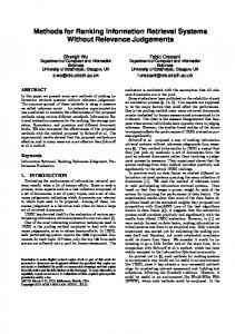
Figure 2. (a) Histogram of absolute weight values for different classifiers (after sorting the dimensions according to the absolute values). L1-LR yields sparser, more skewed weight values which lead to higher retrieval efficiency. (b) Pruning rate of TkP for various classification model and different values of 𝑘 (𝑘 = 10, 3000).

20

Precision @ 10 (%)

average histogram of weight absolute values in figure 2(a). The average histogram for each classification model was obtained by first sorting the weight absolute values for each query in descending order and then normalizing by the largest absolute value so that the largest absolute value is 1. For this experiment we chose 𝐵 = 1000 for the FGM model. We can see that although for this setting the weight vectors learned by FGM are on average more sparse than those produced by L1-LR, the normalized absolute values of the L1-LR weights decay much faster. TkP benefits from the presence of these highly skewed weight values to produce more aggressive pruning. Figure 2(b) shows the average proportion of database pruned by the top-𝑘 method as a function of iteration number (𝑑) for 𝑘 = 10 and 𝑘 = 3000. As anticipated, a smaller value of 𝑘 allows the method to eliminate more images from consideration at an early stage. We now turn to study the effect of parameters 𝐷′ , 𝑣, 𝑤 on the efficiency and accuracy of AR. Figure 3 shows retrieval speed and precision obtained by varying 𝑣 and 𝑤 for 𝐷′ ∈ {128, 256, 512}. Increasing the dictionary size (𝑤) reduces the quantization error while raising the quantization time: note the slightly better accuracy but higher search time when we move from parameter setting (𝐷′ = 512, 𝑣 = 256, 𝑤 = 26 ) to (𝐷′ = 512, 𝑣 = 256, 𝑤 = 28 ). The number of sub-blocks (𝑣) critically affects the retrieval time: reducing 𝑣 lowers a lot the search time but causes a drop in accuracy. Finally, note how 𝐷′ impacts the accuracy since it affects both the number of parameters in the classifier as well as the projection error: using a large 𝐷′ is beneficial for accuracy when 𝑣 and 𝑤 are large; however, when there are few cluster centroids or the number of subblocks is small, lowering 𝐷′ improves precision since this mitigates the quantization error.

v=256, w=26

15 v=256, w=28 10

v=128, w=28 6

v=64, w=2 5

D’=512 D’=256 D’=128

v=16, w=28 0 0

0.02 0.04 0.06 0.08 Search time per query (seconds)

0.1

Figure 3. Effects of parameters 𝐷′ , 𝑣, 𝑤 on the accuracy and search time of AR for the ILSVRC2010 data set. A small 𝑣 implies faster retrieval at the expense of accuracy. A larger 𝑤 reduces the quantization error at a small increase in search time. Reducing 𝐷′ decreases the VC-dimension and increases the PCA projection error, thus causing a drop in accuracy when 𝑣 and 𝑤 are large.

Finally, we also ran an experiment simulating real-world usage of an object-class retrieval system where a user may provide a positive training set but no negative set. In such case one can use a “background” set for the negative class. Here we used as negative examples 𝑛− = 999 images randomly sampled from all categories, thus possibly containing also some true positives. As expected, we found the precisions of the L1-LR and L2-SVM classifiers to be nearly unchanged by the few incorrectly labeled examples: precisions at 10 in this case are 18.75% and 22.55%, respectively.

35

Precision @ 10 (%)

30 25 20

AR L2−SVM TkP L1−LR TkP L2−SVM Inverted index L1−LR Inverted index L2−SVM

15 10

L1-LR L2-SVM FGM LP-𝛽 precision@25 28.2% 30.2% 29.6% 32.8% training time (seconds) 0.044 0.028 11.04 253.7 Table 1. Caltech256 evaluation: precision at 25 and training time for both the state-of-the-art LP-𝛽 classifier as well as our linear classifiers trained on binary classemes. The training set sizes are 𝑛+ = 50 and 𝑛− = 255. The number of true positives in the − = database is 𝑛+ 𝑡𝑒𝑠𝑡 = 25 and the number of distractors are 𝑛 6400. The precisions of these simple linear models approach the accuracy of the LP-𝛽 classifier which is recognized as one of the best object classification systems to date.

5 0 0

50 100 Search time per query (seconds)

150

Figure 4. Search time versus precision at 10 for the 10-million ImageNet data set. For each query class, there are 𝑛+ 𝑡𝑒𝑠𝑡 = 450 positive images and 𝑛− 𝑡𝑒𝑠𝑡 = 9, 671, 611 distractors in the database.

Retrieval results on ImageNet (10M images). We now present results on the 10-million ImageNet dataset [5] which encompasses over 15,000 categories (in our experiment we used 15,203 classes). We used 400 randomly selected categories as query classes. For each of these classes we capped the number of true positives in the database to be 𝑛+ 𝑡𝑒𝑠𝑡 = 450. The total number of distractors for each query is 𝑛− 𝑡𝑒𝑠𝑡 = 9, 671, 611. We trained classifiers for each query category using a training set consisting of 𝑛+ = 10 positive examples and 𝑛− = 15, 202 negative images obtained by sampling one training image for each of the negative classes. We omit from this experiment the FGM model as its training time is over 300 times longer than the time needed to learn the L1-LR or L2-SVM classifier and thus its use on such a large scale benchmark is difficult (as a reference, learning a L1-LR or an L2-SVM classifier for a query category in this experiment takes around 2 seconds). The results are summarized in figure 4, once again in the form of retrieval time versus precision at 10. We can see that on this data set, AR and TkP provide clearly the best accuracy-speed tradeoff, with AR producing slightly better accuracy. Note that near peak-precision with these methods is achieved for an average retrieval time of just a couple of seconds. Here we report search time of TkP for 𝑘 = 10, but we found that when setting 𝑘 = 3000 the retrieval time of TkP increases by only roughly 35% compared to the case 𝑘 = 10. In this figure we are also including the retrieval times obtained with a simple architecture of inverted lists, with each list enumerating the images containing one particular classeme. Retrieval with inverted files obviously yields the same accuracy as TkP but it is more than 7 times slower. Interestingly, AR achieves slightly better accuracy than L2SVM with inverted file indexing. This is probably due to the

PCA preprocessing (which is not used for L2-SVM) which carries out a form of additional regularization on the classifier. This turns out to be beneficial, at least when 𝐷′ is kept large enough. We would like also to comment on the memory usage. The inverted file architecture requires the most space. We represented the image IDs in inverted files using one byte per image: we achieve this by storing only ID displacements (which in our experiment happened to be always smaller than 255) between consecutive images in the list. Despite this clever encoding, the total storage requirement for the 10M data set was roughly 9GB. TkP was implemented using a bit map of all classemes for all images which takes a space of (2659/8) × 𝑁 bytes for a database containing 𝑁 images, which in this case amounts to about 3GB. AR is the most space-efficient: it requires only 𝑣 log2 𝑤 bits to represent each image using vector quantization and the cluster centroids are stored in only 𝐷′ 𝑤 real values. Thus on the 10M data set, the memory usage of AR was only 1.8GB when using 𝑣 = 256, 𝑤 = 26 . This is clearly the most scalable approach in term of memory usage. Object-class retrieval accuracy on Caltech256. Our choice of retrieval models and features was primarily motivated by computational complexity constraints. Thus, a natural, legitimate question is: how much accuracy have we sacrificed for the sake of this efficiency? We answer this question by comparing the retrieval accuracy of our approaches with the state-of-the-art class-recognition system of Gehler and Nowozin [8], which has been shown to produce the best categorization results to date on several recognition benchmarks. This classifier combines non-linear kernel distances computed from multiple feature descriptors. Its high computational complexity and large feature storage requirements makes it impossible to use in large image databases such a those considered in this paper. Thus, we carry out our comparison on the small Caltech256 data set. We use as low-level features for LP-𝛽 the same 13 descriptors that were used to learn the classemes [26], so as to have a comparison between methods on common ground. We

train the retrieval models on each Caltech256 class separately by choosing 𝑛+ = 50 positive examples of the query category and 𝑛− = 255 negative examples obtained by sampling one image from each of the other categories. We report the precision on ranking a database of 6,400 images − including 𝑛+ 𝑡𝑒𝑠𝑡 = 25 true positives and 𝑛𝑡𝑒𝑠𝑡 = 6, 375 distractors obtained by choosing 25 examples from each of the other 255 classes. Table 1 shows that our simple retrieval models applied to binary classeme vectors achieve accuracy comparable to that of the much more computationally expensive LP-𝛽 classifier and are several orders of magnitude more efficient to train as well as test.

8. Discussion We have presented models and algorithms that enable near-instantaneous novel class recognition and search in databases containing several million images with accuracy approaching that of the best known categorization systems. Such scalability is achieved by borrowing tools from information retrieval such as small (but highly-informative) binary codes to represent documents, sparse retrieval models, and algorithms for approximate distance calculation. While such tools have been previously exploited for near-duplicate image detection and for search of object instances we believe we are the first to adapt them to the problem of object class recognition in large collections. Additional material including software and data used for our experiments may be obtained from [1].

Acknowledgements We are grateful to Alessandro Bergamo for help with the experiments. Thanks to Herv´e J´egou for providing code of the product quantization method. This research was funded in part by Microsoft and NSF CAREER award IIS0952943.

References [1] http://vlg.cs.dartmouth.edu/objclassretrieval. 8 [2] A. Berg, J. Deng, and L. Fei-Fei. Large scale visual recognition challenge, 2010. http://www.imagenet.org/challenges/LSVRC/2010/. 5 [3] O. Chum, J. Philbin, and A. Zisserman. Near duplicate image detection: min-hash and tf-idf weighting. In BMVC, 2008. 1, 2 [4] N. Dalal and B. Triggs. Histograms of oriented gradients for human detection. In CVPR, 2005. 1 [5] J. Deng, W. Dong, R. Socher, L. Li, K. Li, and L. Fei-Fei. Imagenet: A large-scale hierarchical image database. In CVPR, 2009. 5, 7 [6] R.-E. Fan, K.-W. Chang, C.-J. Hsieh, X.-R. Wang, and C.-J. Lin. Liblinear: A library for large linear classification. J. of Machine Learning Research, 9:1871–1874, 2008. 3

[7] A. Farhadi, I. Endres, D. Hoiem, and D. Forsyth. Describing objects by their attributes. In CVPR, 2009. 1 [8] P. Gehler and S. Nowozin. On feature combination for multiclass object classification. In ICCV, 2009. 1, 7 [9] K. Grauman and T. Darrell. Pyramid match hashing: Sublinear time indexing over partial correspondences. In CVPR, 2007. 2 [10] T. Hastie, R. Tibshirani, and J. Friedman. The Elements of Statistical Learning. Springer New York Inc., 2001. 4 [11] P. Jain, B. Kulis, and K. Grauman. Fast image search for learned metrics. In CVPR, 2008. 2 [12] H. J´egou, M. Douze, and C. Schmid. Product quantization for nearest neighbor search. IEEE Transactions on Pattern Analysis & Machine Intelligence, 33(1):117–128, 2011. 4 [13] H. J´egou, M. Douze, C. Schmid, and P. P´erez. Aggregating local descriptors into a compact image representation. In CVPR, 2010. 4, 5 [14] B. Kulis and K. Grauman. Kernelized locality-sensitive hashing for scalable image search. In ICCV, 2009. 2 [15] C. H. Lampert, H. Nickisch, and S. Harmeling. Learning to detect unseen object classes by between-class attribute transfer. In CVPR, 2009. 1 [16] S. Lazebnik, C. Schmid, and J. Ponce. Beyond bags of features: Spatial pyramid matching for recognizing natural scene categories. In CVPR, 2006. 1 [17] E. P. X. Li-Jia Li, Hao Su and L. Fei-Fei. Object bank: A high-level image representation for scene classification semantic feature sparsification. In NIPS, 2010. 2 [18] D. Lowe. Distinctive image features from scale-invariant keypoints. Int. Jrnl. of Computer Vision, 60(2):91–110, 2004. 1 [19] C. D. Manning, P. Raghavan, and H. Schutze. Introduction to Information Retrieval. Cambridge Univ. Press, 2008. 2 [20] D. Nist´er and H. Stew´enius. Scalable recognition with a vocabulary tree. In CVPR, 2006. 1, 2 [21] J. Philbin, O. Chum, M. Isard, J. Sivic, and A. Zisserman. Lost in quantization: Improving particular object retrieval in large scale image databases. In CVPR, 2008. 1, 2 [22] G. Shakhnarovich, T. Darrell, P. Indyk, and editors. NearestNeighbors methods in Learning and Vision: Theory and Practice. MIT Press., New York, NY, USA, 2006. 2 [23] J. Sivic and A. Zisserman. Video Google: A text retrieval approach to object matching in videos. In ICCV, 2003. 1, 2 [24] M. Tan, L. Wang, and I. W. Tsang. Learning sparse svm for feature selection on very high dimensional datasets. In ICML, 2010. 3 [25] A. Torralba, R. Fergus, and Y. Weiss. Small codes and large image databases for recognition. In CVPR, 2008. 1 [26] L. Torresani, M. Szummer, and A. Fitzgibbon. Efficient object category recognition using classemes. In ECCV, 2010. 1, 7 [27] L. Torresani, M. Szummer, and A. W. Fitzgibbon. Learning query-dependent prefilters for scalable image retrieval. In CVPR, 2009. 2 [28] Y. Weiss, A. Torralba, and R. Fergus. Spectral hashing. In NIPS, 2008. 2