Jul 18, 2013 - ally cheap tomography scheme which scales polynomially in the system ..... with P1[α] â C1ÃD1 , PN [α] â CDN Ã1, and Pi[α] â. CDiÃDi+1 for ...
Scalable Reconstruction of Density Matrices T. Baumgratz,1, 2 D. Gross,3 M. Cramer,1, 2 and M.B. Plenio1, 2 1
Institut f¨ ur Theoretische Physik, Albert-Einstein-Allee 11, Universit¨ at Ulm, 89069 Ulm, Germany Center for Integrated Quantum Science and Technology, Universit¨ at Ulm, 89069 Ulm, Germany 3 Physikalisches Institut, Hermann-Herder-Straße 3, Albert-Ludwigs Universit¨ at Freiburg, 79104 Freiburg, Germany
arXiv:1207.0358v2 [quant-ph] 18 Jul 2013
2
Recent contributions in the field of quantum state tomography have shown that, despite the exponential growth of Hilbert space with the number of subsystems, tomography of one-dimensional quantum systems may still be performed efficiently by tailored reconstruction schemes. Here, we discuss a scalable method to reconstruct mixed states that are well approximated by matrix product operators. The reconstruction scheme only requires local information about the state, giving rise to a reconstruction technique that is scalable in the system size. It is based on a constructive proof that generic matrix product operators are fully determined by their local reductions. We discuss applications of this scheme for simulated data and experimental data obtained in an ion trap experiment.
The complexity of many-body systems is one of the most intriguing, but at the same time daunting, features of quantum mechanics. The curse of dimensionality, namely the exponential growth of the descriptive complexity of even pure states, is a property of quantum mechanics which clearly distinguishes it from classical physics. Therefore, in general, the number of variables required to uniquely determine a quantum state increases in accordance with the growth of the Hilbert space exponentially. Quantum state tomography addresses the problem of completely characterizing a state of a physical system by measuring a complete set of observables that determine the state uniquely [1]. As the complexity of quantum operations implemented in laboratories steadily increases [2–5], the demand for a reliable and scalable tomography [6, 7] of prepared states is high and of considerable importance for the future of quantum technologies. The ability to store and manipulate interacting quantum many-body systems, such as linearly arranged ions in an ion trap, enhanced rapidly during the last years. Soon, if not already, the number of particles controllable in such systems will cross the threshold for which conventional methods of full quantum state tomography fail due to both the limited time that is realistically available for the experiment and the limitations to the resources that are available for the classical post-processing of the experimental data [2]. Further, while most experiments have so far focused on the controlled creation of pure states and scalable reconstruction methods have been tailored to the pure setting [6, 7], experimental simulations of open system dynamics have begun to emerge [8], calling for efficient tomography of mixed states. The experimental time requirement is defined by the total number of measurements which have to be done to reconstruct the state faithfully; i.e., one has to consider the system size and the number of repetitions to obtain sufficient statistics [9]. The post-processing resources are determined by the individual tomography scheme and in particular by the representation of the state. Clearly, full quantum state tomography where the state is rep-
resented by an exponentially large number of variables will require an exponentially increasing computational power and is hence infeasible already for, e.g., trapped ion experiments available today [4]. But many naturally occurring quantum states and many states of interest for quantum information tasks are completely characterized by a number of variables scaling moderately in the number of particles: ground states of gapped local Hamiltonians [10–12], thermal states of local Hamiltonians [12, 13], the W state, the GHZ state, and cluster states are all matrix product operators (matrix product states if they are pure) of low dimension, or very well approximated by them. These states are parametrized by a linear number of matrices of low bond-dimension. The key insight here is not that these states are matrix product operators or states (any state is a matrix product operator, respectively state) but that the matrix dimension is low, in particular independent of the system size. This solves one issue concerning the post-processing side of the problem mentioned above as these states may be stored efficiently on a classical computer. On the other hand, as we will see, generic matrix product operators are not only completely determined by a linear number of local observables but may also be efficiently reconstructed from such local measurements, which makes the formalism we present here a powerful tool for quantum state tomography of mixed states [14]. Recently, it has been demonstrated that the reconstruction of pure quantum states for large systems can be possible with the knowledge of local information only [6]. The scheme presented in the latter reference relies on an efficient version of an iterative method first introduced in the context of matrix completion. While the original method comes with a convergence proof, this guarantee is lost in the efficient version. Here, we take a different approach, which works provably under a mild technical assumption on the state to be reconstructed and is not restricted to pure states. We present extensive numerical results for states not meeting the assumption guaranteeing uniqueness of the reconstructed density matrix. In this manuscript we consider N d-level subsystems aligned
2 in a one-dimensional geometry, e.g., a chain of qubits (d = 2). The aim is to reconstruct a mixed state %ˆ from local information only. The local information we have in mind are estimates to all reductions of the state to a fixed number R of contiguous sites. These may be obtained by estimating the expectation values of an informationally complete set of observables on the R sites. Note that we do not require the estimates to the reductions to be states; i.e., empirical estimates to the expectation values of local observables suffice and post-processing such as maximum likelihood estimation is not required. As R is fixed, this corresponds to an experimental effort that is linear in the system size N . We present a computationally cheap tomography scheme which scales polynomially in the system size N and succeeds provably under a certain technical invertibility condition on %ˆ. We demonstrate numerically and at the hand of experimental data (a W state on 8 qubits created in an ion trap experiment [2]) that it still works well when this condition is not necessarily met. We begin our exposition of the tomography scheme by introducing some notation. We denote the to-bereconstructed state by %ˆ. The input to the reconstruction scheme are estimates of expectation values which completely specify all reductions of %ˆ to R contiguous sites. We denote these reductions by %ˆk , k = 1, . . . , N − R + 1. Put mathematically, %ˆk = tr{1,...,k−1}∪{k+R,...,N } [ˆ %], i.e., the trace over all but the R sites {k, . . . , k + R − 1}. (α) Now let {Pˆi }α=1,...,d2 be a complete operator basis for the site i. A common choice for spin-1/2 particles is √ √ √ (1) (2) (3) given by Pˆi = 1i / 2, Pˆi = σ ˆix / 2, Pˆi = σ ˆiy / 2, √ (4) Pˆi = σ ˆiz / 2, i.e., the orthonormal Pauli spin basis. We may then write X (α ) (αR ) � ˆ (α1 ) (αR ) %ˆk = Pˆk 1 · · · Pˆk+R−1 P · · · Pˆk+R−1 , (1) %ˆ k α1 ,...,αR
i.e., the %ˆk are completely specified by the local expecta(α ) (αR ) (α ) (αR ) tion values hPˆk 1 · · · Pˆk+R−1 i%ˆ = tr[ˆ %Pˆk 1 · · · Pˆk+R−1 ], estimates to which are the input to our tomography scheme. The %ˆk completely specify the state %ˆ if a certain technical invertibility condition is met. The proof is constructive and gives an explicit method for obtaining %ˆ from the %ˆk . It is partly inspired by the characterization of finitely correlated states (as opposed to C ∗ -finitely correlated states) on infinite spin chains as described in the early literature [15, Prop. 2.1]. In addition to the fact that we are working in a finite and non-translation invariant setting, the main novel technical point here is that we only use local information, provided by the %ˆk . To state the invertibility condition, we first need to establish some notation. We collect the N sites of the one-dimensional system in the set N = {1, . . . , N }. For I ⊂ N , we define the complex vector spaces VI spanned by nY o (α ) Pˆi i . (2) 2 i∈I
αi =1,...,d
1
···
k ···
l ··· k ··· k + r I
N
J
··· ···
N
FIG. 1: Definition of the sets N = {1, . . . , N } and I, J ⊂ N . ˆ = trJ [X ˆO ˆ I∪J ] maps operators X ˆ The linear map EIJ (X) (e.g., observables) living on set J into operators on set I by ˆ (e.g., the state) to I ∪ J . means of the reductions of O
ˆ ∈ VN and I, J ⊂ N we define the linear For given O J map EI : VJ → VN \I as ˆ 7→ E J (X) ˆ = trN \I [X ˆ O]. ˆ X I
(3)
We note that the map EIJ depends only on the reduction ˆ I∪J = trN \I∪J [O] ˆ of O ˆ to sites I ∪ J as O ˆ = trJ [X ˆO ˆ I∪J ]; EIJ (X)
(4)
this is illustrated in Fig. 1. Note that from now on we will only consider cases where I ∪ J is connected.
Definition 1 (Invertibility) Let l, r ∈ N, 2 ≤ l + r ≤ ˆ is such that for all k ∈ N, l ≤ k ≤ N − r − 1, N − 2. If O the equality h i h i {k+1,...,k+r} {k+1,...,N } rank E{k−l+1,...,k} = rank E{1,...,k} (5) ˆ (l, r)-invertible. holds, we call O We may now state the main theorem, a proof of which may be found in Sec. A of the Appendix. Theorem 1 Let l, r ∈ N such that 2 ≤ l + r ≤ N − 2. ˆ ∈ VN be (l, r)-invertible. Then, for all X ˆ i ∈ V{i} , Let O the equality ˆ1 · · · X ˆ N O] ˆ = trN [X ˆ1 · · · X ˆ l Yˆl O] ˆ trN [X
(6)
holds. Here, the Yˆl ∈ V{l+1,...,l+r} are recursively defined ˆ N −r+1 · · · X ˆ N and as follows. We set YˆN −r = X � � ¯ {k,...,k+r−1} E {k,...,k+r} (X ˆ k Yˆk ) Yˆk−1 = E (7) {k−l,...,k−1} {k−l,...,k−1} for k = l + 1, . . . , N − r. Here, the bar indicates the Moore-Penrose pseudoinverse. ˆ to sites Note that, for Eq. (6) the reduction of O {1, . . . , l + r} is needed; for the inverse we require the ˆ to sites {k − l, . . . , k + r − 1}, and for reduction of O {k,...,k+r} ˆ k Yˆk ) we require the reduction of O ˆ to sites E{k−l,...,k−1} (X {k − l, . . . , k + r}. Hence, expectation values of the form ˆ1 · · · X ˆ N O] ˆ are completely specified by reductions trN [X ˆ of O to the sites {k − l, . . . , k + r}, k = l + 1, . . . , N − r,
3
αk+R−1 ˆ tr[Pˆkαk · · · Pˆk+R−1 O],
αi = 1, . . . , d2 ,
(8)
for all k = 1, . . . , N − R + 1. One can prove that a vast majority of matrix product operators fulfil the invertibility condition; i.e., a vast majority of matrix product operators may be reconstructed from local reductions alone (see Sec. B of the Appendix for a technical proof). As noted above, practically relevant states are (well approximated by) matrix product operators of low dimension; i.e., we expect the scheme to work for a large class of mixed states. Now, of course, experimentally, the exact expectation values even for states satisfying the invertibility condition are only known to within a certain statistical error (e.g., the estimated standard deviation of the mean after a finite number of measurements). This error propagates into the singular val{k,...,k+r−1} ues of the map E{k−l,...,k−1} . As this map needs to be inverted, even small errors on singular values close to zero will lead to a large error in the reconstruction. This issue may be avoided by using stochastic robust approximation techniques [16–18] (see Sec. C of the Appendix for technical details). Before we apply the reconstruction scheme to experimental data, we present numerical results for states that do not necessarily fulfil the invertibility condition and for which the local expectation values are subject to inevitable statistical noise. We restrict our attention to qubits d = 2, and illustrate the behaviour of the tomography scheme for thermal states of the Ising Hamiltonian at its quantum critical point ˆ =− H
N −1 X i=1
x σ ˆix σ ˆi+1 −
N X
σ ˆiz .
(9)
i=1
We obtain the thermal states by an imaginary time evolution [19, 20] using the time evolving block decimation algorithm (TEBD). We simulate the measurements in the following way. We first compute the exact lo(α ) (αR ) cal expectation values pkα1 ,...,αR = hˆ σk 1 · · · σ ˆk+R−1 i%ˆ, αi = 0, x, y, z, for all k. Statistical noise is then simulated by adding random numbers (drawn from a Gaussian distribution with zero mean and standard deviation σ) to them. The resulting p¯kα1 ,...,αR then serve as the input to our reconstruction scheme. We compare the reconstructed state %ˆrec to the exact state %ˆ by computing the Hilbert-Schmidt norm difference D (ˆ %, %ˆrec ) = kˆ %rec − %ˆk2 /kˆ %k2 . To obtain meaningful results, we have rescaled the norm such that the deviations are measured in units of kˆ %k2 , the natural length scale of the state to be learned. In Fig. 2, we show the norm difference for the exact and the reconstructed states as a function of the system size N and the error σ. It indicates that, for given
0.08 D (ˆ ̺, ̺ˆrec)
i.e., by all reductions to R = r + l + 1 contiguous sites. ˆ i to be the basis operators Pˆ αi , this By choosing the X i ˆ may be fully reimplies that (l, r)-invertible operators O constructed from their reductions to R consecutive sites, which is the same as knowing the expectation values
0.06 0.04 0.02 0.00 40
32 N
24
16
8
0.003 σ 0.000
0.007
0.010
FIG. 2: Quality of our reconstruction scheme for thermal states of the Ising Hamiltonian in Eq. (9) for β = 5 and R = 5, i.e., the state is reconstructed from local expectation values on five consecutive sites. For each pair (N, σ), the plot shows the mean of the norm difference obtained from 100 realizations and renormalized by the purity of the exact state, i.e. D (ˆ %, %ˆrec ) = kˆ %rec − %ˆk2 /kˆ %k2 . This corresponds to 100 experiments, each of which carries an uncertainty of σ about the local expectation values.
N , the error D (ˆ %, %ˆrec ) scales roughly as σ; similarly, for given σ, it scales roughly as N . In Sec. D of the Appendix we provide further numerical experiments analysing the performance of the algorithm for thermal states of random next-neighbour Hamiltonians and mixed states obtained by tracing out parts of a matrix product state in a larger Hilbert space. Again, these numerical results suggest that the scaling of our scheme is polynomial in both N and σ. Let us finally apply the reconstruction scheme to experimental data obtained in an ion trap experiment in a full quantum state tomography setting. The considered state is a W state implemented on N = 8 qubits with local phases [2], i.e., � |W (φ)i = |0 . . . 001i + eiφ1 |0 . . . 010i+ (10) � √ + . . . + eiφN −1 |1 . . . 000i / N . The available experimental data are the set of relative frequencies corresponding to 100 measurements in each of the 3N different basis rotations (measurements along the X, Y , and Z directions). From these, we obtain maximum likelihood estimates to the reduced density matrices on all blocks of R sites [21]. As described in the Appendix, we apply a stochastic robust approximation technique to avoid difficulties in ill-conditioned inversion problems making use of the Fisher information matrix of the local estimates [21]. Let us stress that the input to the reconstruction scheme are merely the relative frequencies corresponding to the measurements on all subsystems of R contiguous sites and the total number of measurements. Absolute values of the reconstructed density matrices for R = 3 and R = 5 along with the maximum likelihood estimate obtained in the full tomography procedure [2] are presented in Fig. 3. Comparing the
4
(a)
|ˆ �rec | 0.10 (b) 0.08 0.06 0.04 0.02 0.00
(c)
2N
2N
...
..
.
2 1 12
FIG. 3: Absolute value |ˆ %rec | of the corresponding reconstructed density matrix of the experimentally realized W state. (a): Reconstructed operator using the scheme described in this manuscript where the reductions to R = 3 sites are known. (b): Estimate with R = 5 sites. (c): Maximum likelihood estimate of full quantum state tomography (see also [2]). The numbers 1, 2, . . . , 2N denote the entries of the density matrix %ˆrec .
maximum likelihood estimate with our results we find for the renormalized Hilbert-Schmidt norm difference D(ˆ %ML , %ˆrec ) = 0.087 for R = 3 and D(ˆ %ML , %ˆrec ) = 0.012 for R = 5. For the full quantum state tomography experiment, maximizing the fidelity of the maximum likelihood estimate with respect to the local phases of a pure W state yields f = hW (φopt )|ˆ %|W (φopt )i = 0.722 [2]. With the matrix product operator scheme we achieve a fidelity of f = 0.688 for R = 3 and f = 0.718 for R = 5 with respect to the optimal W state |W (φopt )i revealing that the main contribution in our estimates stems from the same |W (φopt )i as in [2]. We are only using local information and hence a local addressing of the ions in the trap is sufficient, resulting in the linear scaling of the scheme with the number of constituents. Further, the full maximum likelihood algorithm uses a huge amount of resources since it requires the storage and manipulation of 6N measurement operators resulting in a time consuming post-processing. In contrast, our reconstruction takes about one second on a laptop given the local maximum likelihood estimates and the corresponding Fisher information matrices [21].
In this work we have presented a scheme to reconstruct mixed states from local measurements efficiently. We have shown that, in principle, all states may be reconstructed from reductions to contiguous sets of sites alone and that the reconstruction is efficient with respect to the measurement time and the post-processing resources for practically relevant states. It should be noted, however, that our rigorous performance guarantees apply only when the model assumption of an essentially onedimensional structure is justified. As is the case for most statistical estimators, the scheme is not suitable for model selection; i.e., it cannot certify unconditionally from data alone that the model is valid. To investigate the latter issue, the impact of statistical noise and the performance of the reconstruction scheme for states that do not necessarily fulfil the condition which guarantees perfect reconstruction have been investigated for simulated states and experimental data in detail. For all simulations the Hilbert-Schmidt norm difference (normalized by the purity of the exact state) between the exact state and the reconstructed state was obtained and the numerical results suggest that the quality of the reconstruction scales algebraically in N and σ. The methods presented here hence pave the way for the reconstruction of mixed states of a large number of qubits. We gratefully acknowledge H. H¨affner for providing experimental data, R. Rosenbach for results of the TEBD algorithm, and K. Audenaert for fruitful discussions. Computations of the TEBD algorithm were performed on the bwGRiD [22]. This work was supported by the Alexander von Humboldt Foundation, the EU Integrated projects QESSENCE and SIQS, the BMBF Verbundprojekt QuOReP, the Excellence Initiative of the German Federal and State Governments (grant ZUK 43), and the Swiss National Science Foundation. Appendix A: Reconstructing Invertible States
In the first section of the Appendix we provide a technical proof that expectation values of product observables with respect to all (l, r)-invertible states are fully determined by expectation values of observables acting only on a subset of the system. These observables can be determined recursively with the knowledge of all reduced density matrices to R = r + l + 1 sites of the considered state. The proof of this lemma provides a scheme to directly determine a matrix product operator representation of the state. Before we proof the main result, let us recall the corresponding theorem in the main text, see theorem 1. Theorem 1 Let l, r ∈ N such that 2 ≤ l + r ≤ N − 2. ˆ ∈ VN be (l, r)-invertible. Then, for all X ˆ i ∈ V{i} , Let O the equality ˆ1 · · · X ˆ N O] ˆ = trN [X ˆ1 · · · X ˆ l Yˆl O] ˆ trN [X
(A1)
holds. Here, the Yˆl ∈ V{l+1,...,l+r} are recursively defined
5 ˆ N −r+1 · · · X ˆ N and as follows. We set YˆN −r = X � � ¯ {k,...,k+r−1} E {k,...,k+r} (X ˆ k Yˆk ) Yˆk−1 = E {k−l,...,k−1} {k−l,...,k−1}
(A2)
for k = l + 1, . . . , N − r. Here, the bar indicates the Moore-Penrose pseudoinverse. Proof. We start by showing that for all k = l + 1, . . . , N − r, Eq. (A2) implies {k,...,k+r−1}
E{1,...,k−1}
{k,...,k+r} ˆ ˆ (Yˆk−1 ) = E{1,...,k−1} (X k Yk ).
(A3)
To this end, we define the linear map φ : {k,...,k+r} {k,...,k+r} ran[E{1,...,k−1} ] → ran[E{k−l,...,k−1} ], where the domain and the range of φ are the ranges of the denoted linear maps, as � {k,...,k+r} � {k,...,k+r} ˆ � ˆ φ E{1,...,k−1} (Z) = tr1,...,k−l−1 E{1,...,k−1} (Z) (A4) {k,...,k+r} ˆ = E{k−l,...,k−1} (Z), {k,...,k+r} ran[E{k−l,...,k−1} ],
i.e., ran[φ] = and therefore, by the rank-nullity theorem, � � {k,...,k+r} {k,...,k+r} dim ker[φ] = rank[E{1,...,k−1} ] − rank[E{k−l,...,k−1} ] {k,...,N }
{k,...,k+r−1}
≤ rank[E{1,...,k−1} ] − rank[E{k−l,...,k−1} ] =0 (A5) due to the invertibility condition, see definition 1 in the ˆ = 0 is equivalent to Zˆ = 0, i.e., main text. Hence, φ(Z) Eq. (A3) is equivalent to � {k,...,k+r} {k,...,k+r} ˆ ˆ � φ E{1,...,k−1} (Yˆk−1 ⊗1) = φ E{1,...,k−1} (X k Yk ) , (A6) which is implied by Eq. (A2). The theorem now follows by induction over k = N − r − 1, . . . , l + 1, starting at k = N − r − 1: the invertibility condition, see definition 1 in the main text, guarantees the existence of YˆN −r−1 ∈ V{N −r,...,N −1} such that {N −r,...,N −1} E{1,...,N −r−1} (YˆN −r−1 )
=
{N −r,...,N }
ˆ1 · · · X ˆ N −r−1 and taki.e., multiplying from the left by X ing the trace over {1, . . . , N − r − 1}, we find ˆ1 · · · X ˆ N O] ˆ = trN [X ˆ1 · · · X ˆ k Yˆk O] ˆ trN [X
(A8)
for k = N − r − 1. Suppose now that this equality holds for l < k ≤ N − r − 1 for some Yˆk ∈ V{k+1,...,k+r} . We now show that it then also holds for l ≤ k −1 ≤ N −r −2. The invertibility condition, see definition 1 in the main text, guarantees the existence of Yˆk−1 ∈ V{k,...,k+r−1} such that {k,...,k+r−1}
ˆ1 · · · X ˆ N O] ˆ = trN [X ˆ1 · · · X ˆ k Yˆk O] ˆ trN [X ˆ1 · · · X ˆ k−1 Yˆk−1 O], ˆ = trN [X
{k,...,k+r} ˆ ˆ (Yˆk−1 ) = E{1,...,k−1} (X k Yk ),
(A9)
(A10)
the desired equality for l ≤ k − 1 ≤ N − r − 2. Appendix B: Generic Matrix Product Operators are Invertible
Here, we show that a vast majority of matrix product operators fulfil the invertibilty condition (see definition 1 in the main text for details). Consider matrix product operators X (α ) (α ) ˆ= O P1 [α1 ] · · · PN [αN ]Pˆ1 1 · · · PˆN N , (B1) α1 ,...,αN
with P1 [α] ∈ C1×D1 , PN [α] ∈ CDN ×1 , and Pi [α] ∈ CDi ×Di+1 for i = 2, . . . , N − 1. We assume w.l.o.g. that (0) Pˆi ∝ 1i for all i = 1, . . . , N . Lemma 1 Let l, r ∈ N such that 2 ≤ l + r ≤ N − 2. ˆ be a matrix product operator as in Eq. (B1). If Let O ˆ tr[O] 6= 0 and for all k ∈ N, l ≤ k ≤ N − r − 1, the sets {Pk−l+1 [αk−l+1 ] · · · Pk [αk ]}αk−l+1 ,...,αk span
{Pk+1 [αk+1 ] · · · Pk+r [αk+r ]}αk+1 ,...,αk+r span
(B2)
CDk−l+1 ×Dk+1 over C and the sets (B3)
CDk+1 ×Dk+r+1 over C, then Oˆ is (l, r)-invertible.
ˆ ∈ V{k+1,...,k+r} , Proof. For X ˆ= X
X αk+1 ,...,αk+r
{N −r,...,N } ˆ N −r YˆN −r ) E{1,...,N −r−1} (X
ˆ N −r X ˆ N −r+1 · · · X ˆ N ), = E{1,...,N −r−1} (X (A7)
E{1,...,k−1}
ˆ1 · · · X ˆ k−1 and taking the multiplying from the left by X trace over {1, . . . , k − 1}, we find
αk+1 αk+r xαk+1 ,...,αk+r Pˆk+1 · · · Pˆk+r ,
(B4)
we find {k+1,...,k+r}
ˆ E{k−l+1,...,k} (X) X ∝ P1 [1] · · · Pk−l [1]Pk−l+1 [αk−l+1 ] · · · Pk [αk ] αk−l+1 ,...,αk
×
X
xαk+1 ,...,αk+r Pk+1 [αk+1 ] · · · Pk+r [αk+r ] αk+1 ,...,αk+r α
=:
X
k−l+1 × Pk+r+1 [1] · · · PM [1]Pˆk−l+1 · · · Pˆkαk
w† Pk−l+1 [αk−l+1 ] · · · Pk [αk ]Xv
αk−l+1 ,...,αk
=: Γ(X),
αk−l+1 × Pˆk−l+1 · · · Pˆkαk
(B5)
6 where the matrix X X= xαk+1 ,...,αk+r Pk+1 [αk+1 ] · · · Pk+r [αk+r ] αk+1 ,...,αk+r
∈ CDk+1 ×Dk+r+1 ,
(B6)
the vectors v = Pk+r+1 [1] · · · PM [1] ∈ CDk+r+1 ×1 ,
w† = P1 [1] · · · Pk−l [1] ∈ C1×Dk−l+1 ,
(B7)
and the mapping Γ : CDk+1 ×Dk+r+1 → V{k−l+1,...,k} . Now, Γ(X) = 0 is equivalent to 0 = w† Pk−l+1 [αk−l+1 ] · · · Pk [αk ]Xv
†
= tr[Pk−l+1 [αk−l+1 ] · · · Pk [αk ]Xvw ]
(B8)
for all αk−l+1 , . . . , αk . Hence, if {Pk−l+1 [αk−l+1 ] · · · Pk [αk ]}αk−l+1 ,...,αk spans CDk−l+1 ×Dk+1 over C, this is equivalent to Xvw† = 0. ˆ 6= 0), this is equivalent Now, as w 6= 0 (implied by tr[O] to Xv = 0. Hence, � ker[Γ] = X ∈ CDk+1 ×Dk+r+1 Xv = 0 , (B9) i.e., the rank of Γ is equal to � Dk+1 Dk+r+1 − dim X ∈ CDk+1 ×Dk+r+1 Xv = 0 . (B10) Now, if {Pk+1 [αk+1 ] · · · Pk+r [αk+r ]}αk+1 ,...,αk+r spans
CDk+1 ×Dk+r+1 over C, we have
{k+1,...,k+r}
ran[E{k−l+1,...,k} ] = ran[Γ],
(B11)
{k+1,...,k+r}
i.e., the rank of E{k−l+1,...,k} is equal to � Dk+1 Dk+r+1 − dim X ∈ CDk+1 ×Dk+r+1 Xv = 0 . (B12) ˆ 6= 0), we may set v 1 = v As v 6= 0 (implied by tr[O] and assume that there are vectors v i ∈ CDk+r+1 ×1 , i = 2, . . . , Dk+r+1 , such that {v i }i=1,...,Dk+r+1 is an orthogonal basis for CDk+r+1 ×1 . Letting {ui }i=1,...,Dk+1 an orthogonal basis for CDk+1 ×1 , we may write Dk+1 Dk+r+1
X=
X
X
i=1
j=1
xi,j ui v †j ,
(B13)
i.e., 0 = Xv = Xv 1 is equivalent to 0 = xi,1 for all {k+1,...,k+r} i = 1, . . . , Dk+1 . Hence, the rank of E{k−l+1,...,k} is equal to Dk+1 Dk+r+1 − Dk+1 (Dk+r+1 − 1) = Dk+1 .
(B14)
Finally, {k+1,...,N }
rank[E{1,...,k}
] ≤ Dk+1 .
(B15)
Appendix C: Non-invertible Inputs
The main issue arising when applying the reconstruction scheme to experimental data is that the local reductions are not known exactly. But of course, we may simply use their estimates (e.g. direct inversions of the measurements, maximum likelihood estimates) as an in{k,...,k+r−1} {k,...,k+r} put to compute the maps E{k−l,...,k−1} and E{k−l,...,k−1} . However, as we need to compute the inverse of the former map, already a small uncertainty will lead to a large error in the inverse. This issue can be dealt with the method of stochastic robust approximation [16]. Before we introduce this regularization technique, let us first ease notation a bit. We write (α ) (α ) Pˆi = Pˆk−lk−l · · · Pˆk−1k−1 ,
ˆ i = Pˆ (αk ) · · · Pˆ (αk+r−1 ) , Q k k+r−1
i = 1, . . . , d2l , i = 1, . . . , d2r .
(C1)
Suppose now that one had access to the exact local expectation values. The matrix representation, A, of {k,...,k+r−1} E{k−l,...,k−1} would then be given by {k,...,k+r−1}
ˆ j )] Ai,j = trk−l,...,k−1 [Pˆi E{k−l,...,k−1} (Q ˆ j O]. ˆ = tr[Pˆi Q
(C2)
Instead, we have only access to the noisy version of the ˆ j O]. ˆ Let us denote the resulting matrix by entries tr[Pˆi Q B. The errors in the measurements propagate into errors of the matrix A. In particular, we write B = A + G where the matrix G contains the errors due to imperfect measurements. Now, when applying the reconstruction scheme we have to solve linear equations of the form Bx = e where B is as described above and e is known. Instead of directly inverting this equation, we take possible variations in the matrix B into account, implying that the entries of B are themselves prone to noise and attempting to undo the imperfect measurements. This is done by introducing the matrix G0 and solving the statistical least-squares problem [16] � � argmin E k(B + G0 )x − ek2 (C3) where E denotes the expectation value and we try to annul the errors in B by the random matrix G0 which we assume to be a multivariate Gaussian distributed random matrix with zero mean and covariance matrix C 0 . This minimization problem can be rewritten as [16] � � argmin kBx − ek2 + xT P x (C4)
with P = E[(G0 )T G0 ]. This sort of regularization problems can be solved analytically. The solution is given by �−1 T x = BTB + P B e (C5) where the entries of P are closely related to the covariance matrix C 0 of G0 X X 0 Pk,l = E[G0i,k G0i,l ] = C(i,k),(i,l) . (C6) i
i
7 It remains to find an appropriate model for the covariance matrix C 0 of the assumed error G0 . In the numerical experiments we simulate statistical noise by adding independent random numbers (drawn from a Gaussian distribution with zero mean and standard deviation σ) to the expectation values of (unnormalized) Pauli strings. With this, the covariance matrix is proportional to the identity and taking the√normalization factor into account 0 we find Ck,l = δk,l · σ/ dr+l . Hence Pk,l = δk,l · σ 2 , and the minimization problem reads � � argmin kBx − ek2 + σ 2 kxk2 . (C7) Problems of this form are known as Tikhonov regularizations [16–18] with solution x = B T B + σ2
�−1
B T e.
(C8)
Let us denote the singular values of B by s1 ≥ · · · ≥ smin{d2l ,d2r } such that B = U SV T . Then, the solution of the statistical least-square problem (C3) in this scenario ¯ with B ¯ = V SU ¯ T where S¯ is a diagois given by x = Be nal matrix with entries fi /si and where fi = s2i /(s2i + σ 2 ) is a smoothing factor suppressing the effect of the smallk,...,k+r−1 est singular values of Ek−l,...,k−1 in its inverse. For the real experimental data we perform maximum likelihood locally to obtain estimates of the reduced density matrices. The remaining problem is to find an error model of the expansion coefficients of the maximum likelihood estimate in the Pauli basis, i.e., the entries of the matrix B. These coefficients can be modelled as the parameters which have to be estimated by the maximum likelihood scheme. To obtain an estimate of the error of these real parameters, we compute the Fisher information matrix F [21] for each subset whose inverse gives a lower bound on the covariance matrix of the matrix B (with respect to the positive semidefinite cone). This is known as the Cram´er-Rao lower bound [21]. Note that maximum likelihood estimates saturate this inequality asymptotically for a large number of measurements [21]. Writing B = A + G where G is a random matrix with zero mean the covariance matrix of B is equivalent to the covariance matrix C of G and hence C ≥ F −1
(C9)
where F(i,k),(j,l) = E
�
∂ log L ∂ log L ∂ Bi,k ∂ Bj,l
� (C10)
is the Fisher information matrix with L the likelihood function and where Bi,k denotes one entry of the matrix B, i.e., an expectation value of the maximum likelihood estimate with a normalized Pauli spin basis element. With this, we model the covariance matrix C 0 of the random matrix G0 in (C3) with the inverse of the Fisher information matrix. Hence, the matrices P can be computed for all subsystems and the solution of the local inversion problems are given by Eq. (C5). Finally,
let us stress that with this procedure the input to the reconstruction scheme are solely the relative frequencies of locally complete measurements obtained in the laboratory and the total number of performed measurements. Appendix D: Numerical Experiments
In this section we continue the numerical analysis of the proposed algorithm for simulated states on large system sizes. In the main text we discussed the behaviour of the reconstruction scheme for thermal states of the Ising Hamiltonian at its quantum critical point. As a second numerical experiment let us analyse the behaviour of the algorithm for states which are exactly representable as matrix product operators satisfying the invertibility condition but subject to statistical noise. We pick such matrix product operators at random by generating a matrix product state with bond-dimension D = d where the entries of the matrices defining the states are drawn from a Gaussian distribution with zero mean and standard deviation one. Then, we let these sites interact with an auxiliary system each of dimension d according to the ˆk = e−iHˆ k t for k = 1, . . . , |Naux |, where H ˆ k is a unitary U two-particle interaction Hamiltonian acting on site k and its auxiliary system with entries picked from a Gaussian distribution with zero mean and standard deviation one. Finally, we trace over the |Naux | auxiliary sites to obtain a matrix product operator with bond-dimension D = d2 . From these states, we compute the exact local expectation values pkα1 ,...,αR , αi = 0, x, y, z for all k, simulate the measurements by adding random numbers (drawn from a Gaussian distribution with zero mean and standard deviation σ), and reconstruct the state by means of the noisy local expectation values. Fig. 4 shows the results for different system sizes and different noise levels. Note that the bond-dimension of the estimate is fixed by the number of sites on which measurements are performed, see theorem 1. The larger these blocks (i.e., the larger R), the larger the bond-dimension of the estimate. This close connection between bond-dimension and block size can be seen in Fig. 4: Increasing the block size dramatically increases the accuracy of the estimate, suggesting the experimental strategy: The block size should be increased until a desired accuracy is reached or measurement time runs out, whichever happens first. Again, the numerical results suggest that the scaling of our scheme is polynomial in both, N and σ. Thermal states of random next-neighbour Hamiltonians of the form ˆ = H
N −1 X
i rˆi,i+1
(D1)
i=1 i serve as our last example. Here, the rˆi,i+1 are Hermitian matrices acting on sites i and i + 1 with entries that have real and imaginary part picked from a Gaussian distribution with zero mean and standard deviation one.
8 (a)
(b)
0.020 0.016
0.3
D (ˆ ̺, ̺ˆrec )
D (ˆ ̺, ̺ˆrec )
0.4
0.2 0.1
0.012 0.008 0.004
0.0 32 28 24 20 16 12 N 8
0.000
0.003
0.007
0.010
σ
0.000 32 28 24 20 16 12 N 8
0.000
0.003
0.007
0.010
σ
FIG. 4: Reconstruction errors for randomly chosen matrix product operators as described in the text with |Naux | = N . The ˆ k kop = 1/100 for all k. For each pair (N, σ) we draw 4000 random interaction is weak in a sense that we choose t such that tkH states, simulate one measurement each and reconstruct the state with the disturbed local expectation values. The plot shows the mean values of the renormalized norm differences in dependence on the system size N and the error in the measurements σ. (a) The states are reconstructed with R = 3, i.e. measurements are done on all blocks of three contiguous sites. Here, for given N (σ), the scaling of D (ˆ %, %ˆrec ) is roughly linear in σ (N ). (b) Reconstruction with R = 5. D (ˆ %, %ˆrec ) improves significantly when measuring on larger blocks.
Again, we use the TEBD [19, 20] algorithm to obtain the exact thermal states. For each system size we generate 50 random Hamiltonians and their corresponding thermal states and simulate one experiment for each σ and state. Fig. 5 shows the error of the reconstructions as a function of the error of the measurements for two different system sizes. The densities illustrate the distribution of the error 0.028
D (ˆ ̺, ̺ˆrec )
0.024 0.020 0.016 0.012 0.008 0.004 0.000 0.002
0.004
0.006 σ
0.008
0.010
FIG. 5: Quality of our reconstruction scheme for thermal states of randomly chosen next-neighbour Hamiltonians as in Eq. (D1) with β = 2 and R = 5, i.e. the state is reconstructed from local expectation values on five consecutive sites. Downward-pointing triangles: system size N = 16, upward-pointing triangles: system size N = 32. We generate 50 different random Hamiltonians and compute their corresponding thermal states using the TEBD algorithm. For each state and pair (N, σ), the density plot shows the simulations of one experiment carrying an uncertainty of σ about the local expectation values. Mean values are indicated as triangles.
for the 50 different states while the black arrows indicate the mean.
9
[1] Quantum State Estimation, Lecture Notes in Physics Vol. ˘ a˘cek (Springer, 649, edited by M.G.A. Paris and J. Reh´ Berlin Heidelberg, 2004). [2] H. H¨ affner, W. H¨ ansel, C.F. Roos, J. Benhelm, D. Chekal-kar, M. Chwalla, T. K¨ orber, U.D. Rapol, M. Riebe, P.O. Schmidt, C. Becher, O. G¨ uhne, W. D¨ ur, and R. Blatt, Nature (London) 438, 643 (2005). [3] D. Leibfried, E. Knill, S. Seidelin, J. Britton, R.B. Blakestad, J. Chiaverini, D.B. Hume, W.M. Itano, J.D. Jost, C. Langer, R. Ozeri, R. Reichle, and D.J. Wineland, Nature (London) 438, 639 (2005). [4] T. Monz, P. Schindler, J.T. Barreiro, M. Chwalla, D. Nigg, W.A. Coish, M. Harlander, W. H¨ ansel, M. Hennrich, and R. Blatt, Phys. Rev. Lett. 106, 130506 (2011). [5] X.-C. Yao, T.-X. Wang, P. Xu, H. Lu, G.-S. Pan, X.-H. Bao, C.-Z. Peng, C.-Y. Lu, Y.-A. Chen, and J.-W. Pan, Nat. Photonics 6, 225 (2012). [6] M. Cramer, M.B. Plenio, S.T. Flammia, R. Somma, D. Gross, S.D. Bartlett, O. Landon-Cardinal, D. Poulin, and Y.-K. Liu, Nat. Commun. 1, 149 (2010). [7] D. Gross, Y.-K. Liu, S.T. Flammia, S. Becker, and J. Eisert, Phys. Rev. Lett. 105, 150401 (2010); G. T´ oth, W. Wieczorek, D. Gross, R. Krischek, C. Schwemmer, and H. Weinfurter, Phys. Rev. Lett. 105, 250403 (2010); D. Gross, IEEE Trans. on Inf. Theory, 57, 1548 (2011); M.P. da Silva, O. Landon-Cardinal, and D. Poulin, Phys. Rev. Lett. 107, 210404 (2011); S.T. Flammia and Y.-K. Liu, Phys. Rev. Lett. 106, 230501 (2011); S.T. Flammia, D. Gross, Y.-K. Liu, and J. Eisert, New J. Phys. 14, 095022 (2012); O. Landon-Cardinal and D. Poulin, New J. Phys. 14, 085004 (2012). [8] P. Schindler, M. M¨ uller, D. Nigg, J.T. Barreiro, E.A. Martinez, M. Hennrich, T. Monz, S. Diehl, P. Zoller, and R. Blatt, Nat. Physics 9, 361 (2013). [9] D.F.V. James, P.G. Kwiat, W.J. Munro, and A.G. White, Phys. Rev. A 64, 052312 (2001). [10] M.B. Hastings, J. Stat. Mech. P08024 (2007). [11] M.B. Plenio, J. Eisert, J. Dreißig, and M. Cramer, Phys. Rev. Lett. 94, 060503 (2005). [12] J. Eisert, M. Cramer, and M.B. Plenio, Rev. Mod. Phys.
82, 277 (2010). [13] M.B. Hastings, Phys. Rev. B 73, 085115 (2006). [14] There is of course no contradiction between the exponential speed up of quantum computation and the fact that some states in large ambient spaces can be efficiently handled. Indeed, we believe it is a key contribution of quantum information to develop complementary tools with the eventual aim to decide which states allow for an efficient simulation (like the ones treated here) and which ones do not (e.g., those enabling universal quantum computation). [15] M. Fannes, B. Nachtergaele, and R.F. Werner, Commun. Math. Phys. 144, 443-490 (1992). [16] S. Boyd and L. Vandenberghe, Convex Optimization (Cambridge University Press, Cambridge, England, 2004). [17] J.S. Lundeen, A. Feito, H. Coldenstrodt-Ronge, K.L. Pregnell, Ch. Silberhorn, T.C. Ralph, J. Eisert, M.B. Plenio, and I.A. Walmsley, Nat. Phys. 5, 27 (2008). [18] L. Zhang, H. Coldenstrodt-Ronge, A. Datta, G. Puentes, J.S. Lundeen, X.-M. Jin, B.J. Smith, M.B. Plenio, and I.A. Walmsley, Nat. Photonics 6, 364 (2012). [19] M. Zwolak and G. Vidal, Phys. Rev. Lett. 93, 207205 (2004). [20] To generate the thermal states we use a fourth order Trotter expansion and adjust the step size in the imaginary time evolution to δT = 10−3 for the Ising Hamiltonian and the random next-neighbour Hamitonians, reˆ spectively, i.e., %ˆ = (e−δT H )β/δT /Z. Further, we keep the 100 largest singular values in each decomposition, i.e., approximate the state as a matrix product operator with bond-dimension D = 100. ˘ a˘cek, J. Fiur´ [21] Z. Hradil, J. Reh´ a˘sek, and M. Je˘zek, Lect. Notes Phys. 649, 59-112 (2004). [22] bwGRiD (http://www.bw-grid.de), member of the German D-Grid initiative, funded by the Ministry for Education and Re-search and the Ministry for Science, Research and Arts Baden-W¨ urttemberg.