IEEE TRANSACTIONS ON MICROWAVE THEORY AND TECHNIQUES, VOL. 58, NO. 12, DECEMBER 2010
3749
Scalar Measurement-Based Algorithm for Automated Filter Tuning of Integrated Chebyshev Tunable Filters Nino Zahirovic, Student Member, IEEE, Raafat R. Mansour, Fellow, IEEE, and Ming Yu, Fellow, IEEE
Abstract—A system and method for the automated tuning of coupled resonator tunable filters is presented. The system and method are amenable to integration and are developed for on-board and on-chip automatic tuning of tunable filters without the use of a vector network analyzer and with minimal additional hardware. An analytical coupling matrix-based model of the tuning algorithm is developed to analyze and predict the performance of the tuning algorithm. The tuning model is verified with the automated tuning algorithm operating on a realized tunable filter. Finally, a lowcost hardware prototype for scalar transmission measurement for standalone implementation of the algorithm is also presented. Index Terms—microwave filters, circuit tuning, automated tuning.
I. INTRODUCTION
M
ULTIBAND radios are a topic of significant recent interest due to increased demand for smartphones with global coverage and the sparse allocation of wireless spectrum for cellular applications. Current implementations of multiband radios result in duplicate hardware with a dedicated signal chain for each band. The duplicate hardware results in higher cost and larger circuit area as the number of covered bands increases. A single tunable analog signal chain with software defined baseband processing has the potential to reduce circuit area and result in more flexible and scalable multiband radios. The fixed RF filters in the analog portion of the signal chain are significant stumbling blocks for the consolidation of multiple signal chains. The integration of tunable filters into handheld mobiles is a desirable step to multiband consolidation. The initial technical challenge is in achieving a low-loss tunable filter that is small enough for handheld use. There is considerable research in the area of miniature low-loss tunable filters [1]. However, once miniature tunable filters are made available, there remains the challenge of tuning such filters. The work presented here addresses the problem of integrated filter tuning with a low-cost and highly integrated approach. Manuscript received June 01, 2010; revised August 24, 2010; accepted August 29, 2010. Date of publication November 09, 2010; date of current version December 10, 2010. This work was supported in part by the Natural Sciences and Engineering Research Council of Canada (NSERC) and COM DEV International Ltd. N. Zahirovic and R. Mansour are with the Department of Electrical and Computer Engineering, University of Waterloo, Waterloo, ON, Canada N2L 3G1 (e-mail:
[email protected]). M. Yu is with COM DEV International Ltd., Cambridge, ON, Canada N1R 7H6. Color versions of one or more of the figures in this paper are available online at http://ieeexplore.ieee.org. Digital Object Identifier 10.1109/TMTT.2010.2085791
It is envisioned that the proposed technique may be used as an initial calibration method during band switching of a tunable multiband radio system. The proposed tuning algorithm is computationally efficient and only relies on the measurement of the transmission response of the tunable filter for full calibration/tuning of Chebyshev-class filters. A tunable Chebyshev filter is controlled by a number of frequency and coupling tuning elements. The tuning elements may be any of a number of tunable components such as tuning screws, semiconductor varactors, MEMS switches, BST varactors, etc. The prescribed purpose of each of these tuning elements is the tuning of either a resonator’s center frequency, the coupling between two adjacent resonators, or the external quality factors of the input and output resonators. The problem of tuning a filter is complex because of the high level of interaction between the center frequency of each resonator and the couplings that combine to generate the final filter response. The algorithm proposed here is directed at tuning Chebyshev filters with only center frequency tuning elements. The complexity of filter tuning has led researchers to develop group delay [2], time-domain [3] and fuzzy logic [4] techniques to reduce the complexity of the filter tuning problem. These techniques were all developed for the design and postproduction tuning of coupled resonator filters and rely on both the phase and/or magnitude quantities of the reflection coefficient. A completely automated system was also demonstrated in [5] for the post production tuning of microwave filters using phase and magnitude data measured by a vector network analyzer (VNA). VNAs are costly and relatively large pieces of equipment that are difficult to integrate into embedded devices as shown in Fig. 1(a). The parameter extraction based tuning methods described in [6]–[8] all rely on pole and zero identification of the filter transfer function from the phase data and eventual transcription to the coupling matrix model for tuning and, therefore, require the use of a VNA for filter measurement. Scalar characterization, as shown in Fig. 1(b), is a lower cost option that results in a less precise measurement since full calibration requires vector data. The proposed scalar transmission-based tuning technique described here does not require the use of any directional couplers or quadrature receivers and is therefore highly capable of being monlithically integrated. The approach reduces the required tuning hardware and cost as shown in Fig. 1 and enables the integration of closed-loop tuning with minimal additional hardware. In addition, the components necessary for tuning can all be found in commercial off-the-shelf transceivers resulting in reduced incremental cost as shown in Fig. 1(c).
0018-9480/$26.00 © 2010 IEEE
3750
IEEE TRANSACTIONS ON MICROWAVE THEORY AND TECHNIQUES, VOL. 58, NO. 12, DECEMBER 2010
Fig. 1. Filter measurement configurations with cost comparison. The VNA (vector network analyzer) configuration shown in (a) is the most expensive followed by the SNA (scalar network analyzer) configuration shown in (b). The commercial off-the-shelf hardware configuration shown in (c) is highly amenable to integration. The highlighted blocks in (c) are readily available components in commercial transceivers and can be integrated into a monolithic solution.
A. Algorithm Description The proposed scalar transmission-based tuning algorithm relies on a similar sequential tuning concept as the Hilbert transform-derived group delay tuning method [9], group delay tuning method [2], and the alternating short and open method [10]. The primary concept borrowed from the other sequential tuning techniques is the assumption of minimal loading if there is sufficient separation in center frequency between resonators. Ideally, as in [2] and [10], all detuned resonators are completely short circuited to eliminate the loading effects entirely. A filter with a perfectly shorted resonator will not transmit any signal and, therefore, the techniques of [2] and [10] rely on the mea. The measurement of surement of the reflected signal or the reflected signal requires the use of directional couplers that make integration more difficult. Therefore, as in [9], we create an effective short in the filter by detuning a resonator and mea. suring the magnitude of the transmission characteristic or For example, if it is desired that a filter be tuned to a target frequency, , an effective short of a resonator is realized at by where is ensuring that its resonant frequency is chosen to be large compared to the bandwidth of the filter. A is imposed by the order of the limit on the magnitude of filter and the dynamic range of the tuning hardware. Incomplete detuning results in finite tuning error due to the loading caused by the incompletely shorted resonators. As shown in Section II, the tuning error tends to zero. as The algorithm begins with the assumption that the filter is tuned at an initial center frequency, , and that the desired (target) center frequency is . If is sufficiently large, such that a resonator tuned at appears as an effective short at frequency , then this tuning hop is performed directly; otherwise, an intermediate tuning hop may be required to achieve a particular frequency tuning accuracy. A frequency hop from to proceeds as follows. A tuning hop commences with the position of all the center where frequency tuning elements at the initial state is the state vector containing the position of each of the tuning elements and is the number of resonators. It is assumed that the initial state of the filter has all the tuning
elements set to the same frequency. The filter tuning process is illustrated using Fig. 2 where a coupling-matrix based model is used to illustrate the tuning algorithm. The details of the coupling matrix model are described in Section II. Fig. 2 represents the filter in the lowpass domain with the initial frequency normalized to 0 rad/s as shown in Fig. 2(a) and, therefore, initial . The first resonator is swept from its state vector initial position, , to find the position of the tuning element that results in a maximum of signal transmission through the rad/s as shown in Fig. 2(b). filter at the target frequency A sample filter response with the first tuning element set to the position of maximum transmission at is shown in Fig. 2(b) with the tuning curve used to find the point of maximum transmission shown next to the filter response. The tuning element position resulting in the maximum transmission at is recorded in the target state vector as . The first resonator such that it appears as an is returned to its initial state effective short for the tuning of the subsequent resonators; thus, completing the tuning of the first resonator. The algorithm resumes with the second tuning element being swept to determine , as shown in Fig. 2(c), and so on until the complete target is determined. The tuning state vector hop is completed by positioning all the tuning elements to positions recorded in the target state vector —thus, nominally rad/s as shown in tuning the filter at the target frequency, Fig. 2(d). The tuning curves shown adjacent to the filter response versus tuning elin Fig. 2(b) and (c) are formed as plots of ement state, , at the target frequency . The tuning curves of versus are well behaved containing a single maxima and are, therefore, amenable to peak finding using simple optimization routines. An integrated tunable system would implement the tuning algorithm as follows. A frequency synthesizer, such as the phase locked loop (PLL) of a transceiver, is set to the target frequency, , of the filter. The first tuning element state is swept over its entire state space with the magnitude of transmission being noted over the full sweep. The maximum of transmission is determined and the state of the tuning element at the point of max. The tuning element is reimum transmission is recorded as turned to its starting position . The same process is repeated with each tuning element to find the complete target state vector . Upon completing the process with the final resonator, the target state vector is applied to the filter to set it at the algorithm determined target frequency. The maximum hop is limited by the dynamic range of the filter characterization hardware. The dynamic range of a single chip transceiver implementation would most likely be limited by the isolation between the receive and transmit signal chains since both signal chains would be tuned to the same frequency, . In the case of a single chip transceiver this is on the order of 30 to 40 dB. The isolation between the signal source (PLL) and the receiver effectively sets the noise floor of the transmission measurement. Due to the limitations imposed by the dynamic range of the measurement hardware, the adjacent resonators can only be detuned as far as a signal is still detectable with reasonable fidelity at the output of the filter. Tuning of higher order filters also requires higher dynamic range measurement hardware.
ZAHIROVIC et al.: SCALAR MEASUREMENT-BASED ALGORITHM FOR AUTOMATED FILTER TUNING OF INTEGRATED CHEBYSHEV TUNABLE FILTERS
3751
Fig. 2. The initial filter response using a coupling matrix model for a third order filter with 25 dB return loss is shown in (a). The filter response at the end of each tuning step and the tuning curves when each resonator is tuned are shown in (b) and (c). The plots for resonators 1 and 3 are the same due to symmetry and are shown in (b). The final response after setting the algorithm determined coupling matrix values is shown in (d).
Fig. 3. Coupling matrix model in the normalized lowpass frequency domain. The B elements represent frequency invariant reactances, while R and R are the input and output normalized load resistances and represent the input and output couplings, respectively.
II. THEORY A theoretical basis for the tuning algorithm is developed using a coupling matrix model for a coupled resonator tunable filter [11]. Consider the lowpass prototype of a coupled-resonator filter as shown in Fig. 3. In Fig. 3 the elements labeled are frequency invariant reactances that are traditionally used to permit the modeling of asynchronous filters. In the tunable filter are used to permit model, the frequency invariant reactances the detuning of individual resonators away from the nominal passband. In the bandpass case, the frequency invariant elements introduce a resonance frequency shift to a resonator. In the following analysis, the frequency invariant elements are used to represent the effects of center frequency tuning. The S-parameters of the network in Fig. 3 are expressed in and terms of the coupling matrix as given in (1) with representing the normalized input and output resistances. The matrix is N N with all entries zero except for and as given in (2). The coupling matrix for the network shown in Fig. 3 is given in (3) where is the order of the network and the number of resonators.
Most Chebyshev filters have identical source and load imand, therefore, the subscripts of the pedances with elements of the R matrix are dropped to simplify the following . The frequency variable is repreanalysis where sented by and is equal to where is the lowpass frequency variable. The frequency variable can also be transformed to and, the bandpass domain using (4) where and are the lower and upper cutoff frequencies at the designated return loss, respectively [11]. A filter exhibiting an ideal equal-ripple Chebyshev response has all the diagonal elements of its coupling matrix set to 0.
(1)
.. .
.. .
.. .
..
.. .
.
.. .
..
(2)
.
.. .
.. .
(3)
(4) The coupling matrix given in (3) is augmented to form the by introducing frequency invariant tunable coupling matrix
3752
IEEE TRANSACTIONS ON MICROWAVE THEORY AND TECHNIQUES, VOL. 58, NO. 12, DECEMBER 2010
reactances into the main diagonal of the coupling matrix as given in (5). In (5), is the N N identity matrix and is the . state vector of the tunable filter where The frequency invariant reactances model the tuning elements of the filter and end up on the main diagonal of the tunable . All the elements of the state vector are inicoupling matrix , represents tially set to zero. The initial state, the filter tuned at its initial center frequency . Effectively, the tunable filter bandpass response is normalized to the lowpass domain such that the initial center frequency is normalized to 0 rad/s in the lowpass domain. (5) The tunable coupling matrix of (5) is substituted into the expressions relating the S-parameters and the coupling matrix (1) and yield the S-parameters as a function of the state vector and frequency as given in (6):
errors of imperfect detuning. The error function for a particular element of the tuning state is defined in (8): (8) is the tuning algorithm determined state for the where target frequency, . A. A Quantitative Example of the Modeled Tuning Algorithm The behavior of the tuning algorithm is illustrated with a numerical example based on the tunable coupling matrix presented above. A third order filter with 25 dB return loss is used as the example. The low order filter is typical of what may be encountered in a front-end filter and results in manageable symbolic algebraic solutions in print form. Higher order solutions are still analytical but result in long symbolic expressions. and load matrix are given in (9) The coupling matrix and (10), respectively, for the specific case of this filter example. This synthetic example is identical to the one used in Section I with response curves shown in Fig. 2.
(6) Thus, (6) gives the S-parameters as a function of the state of the filter tuning elements. The effectiveness of the tuning algorithm is now evaluated using the model relating the state of the tunable filter and the S-parameters. The algorithm within the context of the tunable filter model is described as follows. The magnitude of the filter transmission at the target frequency is found by evaluating the magnitude as a function of the state vector at the frequency of or . The maximum of transmission at is found for each resonator by solving the set of independent equations given in (7). The resulting vector is the scalar algorithm-determined target state vector. The superscript designates a value determined by the scalar tuning algorithm. The ideal tuning states are designated with a with the ideal target state vector designated . The tuning error vector is now defined as .
.. .. .. ... (7) The tuning algorithm model of (7) is confirmed to result in analytical solutions up to an arbitrary order. The analytical results of the modeled tuning algorithm serve to illustrate the fundamental limitations of the tuning approach and to aid in determining the bounds on the tuning error. The relationship and the ideal state between the target center frequency vector for perfect tuning is easily solved. A resonator that is desired to have a lowpass normalized resonant frerad/s needs to have . Therefore, quency of . The solution of (7) evaluates the result of the tuning algorithm and captures the systematic
(9)
(10) The squared magnitude response of the transmission coefficient for a third order filter can be expressed as (11), shown at the bottom of the following page, for the outer resonator and middle resonator tuning case tuning case . The outer resonator tuning functions apply to both resonators 1 and 3. In order to find the tuning curves is substituted into the expressions given shown in Fig. 4, in (11) and the magnitude of transmission is plotted versus with the coupling matrix values for and substituted from (9) and (10), respectively. The expressions for the magand for this nitude of transmission versus the values of filter example are given in (12) and (13), respectively, shown at the bottom of the following page. The plot of Fig. 4 indicates that a dynamic range of at least 20 dB is necessary to identify the transmission peak for resonators 1 and 2 at a lowpass hop distance of 5 rad/s. rad/s in freIn the normalized lowpass domain a shift of quency is the result of setting the diagonal elements of the cou. However, it has been noted that the effects pling matrix to of non-ideal detuning will hamper the performance of the algorithm. As seen in Fig. 4, the maxima of transmission at the target rad/s does not occur at the ideal value of frequency of . This highlights the presence of error inherent in the tuning algorithm. Taking the derivatives of the expressions (12) and (13) with and , respectively, and equating them to zero respect to allows expressions for the tuned resonant frequency with respect to target frequency to be developed as given in (14) and (15), respectively, shown at the bottom of the following page. In order to quantify the effects of non-ideal detuning on the proposed tuning algorithm, the tuning error function can be found
ZAHIROVIC et al.: SCALAR MEASUREMENT-BASED ALGORITHM FOR AUTOMATED FILTER TUNING OF INTEGRATED CHEBYSHEV TUNABLE FILTERS
Fig. 4. Tuning curves for elements B and B of the tunable coupling matrix (9). The curves are generated by plotting jS ([B ; 0; 0]; 5)j and ([0; B ; 0]; 5)j as a function of B and B , respectively. These plots are jS analogous to generating a transmission magnitude sweep versus tuner position for f = 5 rad/s.
by taking the difference of the solution of (7) and . The error can be expressed versus target frequency to determine the size of the required step and the expected magnitude of the inherent tuning error using (8). The result of the tuning law (7) for the outer and middle resonators in the case of the example third order filter are listed in (14) and is the algorithm-derived diag(15), respectively, where onal element value as a function of the target frequency . The limit of the expressions (14) and (15) as approaches . Consequently, the tuning error as given in (8) will infinity is . It should also be noted that tend to zero as approaches since the initial center frequency is normalized to 0 rad/s in the
3753
lowpass domain the initial center frequency is always in the lowpass domain. Therefore, the tuning hop magnitude in this example since we are formulating the theory in the normalized lowpass domain. The tuning error for the example filter is plotted with respect for the tuning of the middle resonator to target frequency and end resonator tuning element tuning element and is shown in Fig. 5. The magnitude of the tuning error is shown in Fig. 5 for both the middle and end resonators versus in both the downward and the size of the tuning hop upward tuning directions as shown in Fig. 5(a) and (b), respectively. Fig. 5 shows that initially the tuning error is very small if a small step is made from the initial passband. However, the error increases quickly as the tuning hop distance approaches the vicinity of the band edge of the filter’s initial state where the error caused by adjacent resonators is at a maximum. Therefore, for the assumption of minimal loading to hold true, the hop should be at least a couple of filter bandwidths away to be performed directly. The error can be ensured to be below a certain threshold if the hop size is maintained above a prescribed minimum. The tuning error decreases with the tuning hop distance once the maximum near the initial filter band edge is passed. In Fig. 5(a) two tuning offsets are noted for comparison. Tuning offset (a) is 2 rad/s while tuning offset (b) is 9 rad/s. Both tuning offsets (a) and (b) are in the negative tuning or rad/s and direction with rad/s, respectively. The algorithm-tuned response for tuning offsets (a) and (b) are shown using solid lines in Fig. 6 with . The ideal filter response at rad/s and rad/s are shown with dotted . The comparison in Fig. 6 lines where shows that the response at offset (b) is closer to the ideal dotted
(11) (12) (13)
(14)
(15)
3754
IEEE TRANSACTIONS ON MICROWAVE THEORY AND TECHNIQUES, VOL. 58, NO. 12, DECEMBER 2010
Fig. 6. A lowpass normalized prototype comparison of an ideal third order Chebyshev coupling matrix response and that of a worst case tuned Chebyshev filter using the proposed tuning algorithm with 25 rad/s error. The ideal response is shown with the dotted curves while the algorithm-tuned response is shown with solid lines.
Fig. 5. The magnitude of the tuning error versus frequency offset for tuning in the downward (a) and upward (b) cases. Error curves are shown for both the outer (E ) and middle (E ) resonators.
response than the response at offset (a). The result at offset (a) shows a greater center frequency error compared to offset (b) since it is the result of a smaller tuning hop. In both offsets (a) and (b) the algorithm-tuned filter response errs on the side of the initial center frequency. do not remain In general, the coupling element values constant over all tuning states of the tunable filter state vector as assumed by this model. A filter with constant and is a filter with constant fractional bandwidth. It is often more desirable for a tunable filter to exhibit constant absolute bandwidth over the center frequency tuning range. However, it is noted that many tunable filters exhibit a nearly constant fractional bandwidth making this model fairly accurate in those cases [12]–[14]. The presented analytical model results in a reasonable approximation of the tuning behavior in general and serves as an adequate model to illustrate the concept and limitations of the proposed tuning scheme. III. MEASURED RESULTS Two measurement hardware configurations are presented for the validation of the scalar tuning algorithm. One hardware configuration uses a traditional VNA instrument for both scalar measurement and final filter characterization. The other config-
uration uses a discrete PLL circuit as a continuous-wave signal source and a log-amplifier detector to form a low-cost scalar measurement system. The VNA measurement setup serves to illustrate the accuracy of the tunable filter model and verify the postulates of the tuning algorithm, while the scalar hardware measurement setup serves to demonstrate the capability of a low-cost hardware implementation of the algorithm. A large scale tunable filter is used to demonstrate the performance of the algorithm. The tunable filter is a servo-motorcontrolled evanescent mode coupled rectangular coaxial cavity combline filter. Tuning is accomplished using traditional #4-40 tuning screws that are automatically driven by servo motors through flexible couplings. The same flexible coupling/servo motor configuration was used in [4] to demonstrate post-production filter tuning using automated fuzzy logic techniques. Initialization of the tunable filter hardware is done manually by homing the servo actuators at the lowest possible position (screws inserted as far into the cavity as possible) without shorting the tuning screw to the resonator post. This lowest-most position corresponds to an encoder reading of 0 counts. Turning the motor in the positive direction, so as to increase the encoder count, retracts the screw out of the cavity and increases the resonance frequency of the resonator being tuned. The coaxial resonator tunable filter has a tuning range of 800 MHz (from 4 GHz to 4.8 GHz). The tuning characteristic of the rectangular coaxial resonator versus screw position is simulated in Ansoft HFSS. The tuning screw is modeled as a smooth-walled cylinder with a diameter of 2.72 mm, corresponding to the minimum major diameter of a #4 screw. A parametric simulation was performed using Ansoft HFSS to determine the center frequency tuning characteristic of the cavity and is shown in Fig. 7. The result shown in Fig. 7 is nonlinear. Therefore, in order to ensure a constant frequency resolution across the tuning range, the function shown in Fig. 8 is applied to linearize the response between sweep step and resonator frequency. Fig. 8 is an inversion of the simulated tuning response of Fig. 7. The linearized frequency step characteristic of Fig. 8 was used for both the VNA and scalar measurement hardware configurations.
ZAHIROVIC et al.: SCALAR MEASUREMENT-BASED ALGORITHM FOR AUTOMATED FILTER TUNING OF INTEGRATED CHEBYSHEV TUNABLE FILTERS
3755
Fig. 9. Tuning algorithm model validation setup using a VNA for the measurement of the transmission magnitude response.
Fig. 7. Center frequency tuning characteristic for the center frequency resonator results obtained from simulation using Ansoft HFSS.
Fig. 10. The transmission response sweep versus actuator position step for the three tuning actuators while performing a hop from 4.8 GHz to 4.2 GHz. The maximum of the transmission response for each actuator is selected as the tuned position for 4.2 GHz. Note that a nonlinear step size is used based on the simulated tuning characteristic as shown in Fig. 8.
TABLE I HOP SWEEP CONFIGURATION FOR THE UP-SWEEP AND DOWN-SWEEP PLANS Fig. 8. Encoder position versus tuning sweep step. This curve inverts the tuning characteristic to approximate a linear response between sweep step and resonator frequency.
A. Scalar Measurement Based Tuning Implementation Using a VNA A block diagram of the VNA-based test configuration is shown in Fig. 9. A PC running LabVIEW is used to run the algorithm while the VNA is used to measure the log-magnitude of the transmission response of the filter during the tuning process. During the tuning process, the VNA is used strictly to measure the relative transmission magnitude. After a particular tuning hop is completed, the VNA is returned to its vector measurement state to capture the complete two-port characteristics of the filter. In this fashion, both tuning and response validation is performed in a single physical configuration. The tuning algorithm is tested over two multi-hop scans of the tuning range in the increasing frequency (upward) and decreasing frequency (downward) directions as shown in Table I. The initial frequency position, , for each of the upward hops is set to 4 GHz while the for each of the downward hops is set to 4.8 GHz. During each actuator tuning sweep the VNA is set to continuous wave mode at the target frequency of the hop. Eleven samples of the transmission response are taken over 5.5
ms and averaged for each sample of the transmission magnitude versus actuator position sweep. The actuator tuning sweeps generate the three tuning curves, one for each resonator, as shown in Fig. 10. Once the tuning curves of Fig. 10 are generated for a particular hop, the positions resulting in maximum transmission are selected as the target positions for each resonator and make up the target state vector . The tuning hop is concluded by setting the positions of the actuators to the determined target and the complete tuned two-port response is meapositions sured over the tuning range of the filter and logged as an s2p file. The initial position is returned to and a new is set on the VNA for the next hop. The results of the logged s2p files are shown in Fig. 11 for the target frequencies of 4200 MHz, 4400 MHz, 4600 MHz and 4800 MHz for the up-sweep [Fig. 11(a)] and 4000 MHz, 4200 MHz, 4400 MHz and 4600 MHz for the down-sweep
3756
IEEE TRANSACTIONS ON MICROWAVE THEORY AND TECHNIQUES, VOL. 58, NO. 12, DECEMBER 2010
Fig. 12. The return loss (S ) is plotted for both the up- and down-sweeps of f at 4.2 GHz, 4.4 GHz, and 4.6 GHz. The final center frequency is higher than f in the down-sweep and less than f in the up-sweep as predicted by the model. The responses are nearly symmetrical about f .
Fig. 11. Upward and downward tuning results compared. The transmission response is shown using solid lines while the reflection is shown with dotted lines. (a) Tuning results using a VNA as a scalar network analyzer for tuning and final measurement for f > f . The f is 4 GHz while results are plotted with f at 4.2 GHz, 4.4 GHz, 4.6 GHz, and 4.8 GHz. (b) Tuning results using a VNA as a scalar network analyzer for tuning and final measurement f < f . The f is 4.8 GHz while results are plotted with f at 4 GHz, 4.2 GHz, 4.4 GHz, and 4.6 GHz.
[Fig. 11(b)]. These target frequencies are selected to have non-overlapping responses in the same figure. The scalar algorithm only tunes the center frequency of each resonator. As a result, the return loss shown in Fig. 11 is poor at the low end of the tuning range since the coupling tuning screws were fixed for the duration of testing. The algorithm presented here makes no attempt to tune the coupling and, as a consequence, the return loss is determined by the coupling variation with center frequency. The increase in insertion loss with lower frequency is attributed to a reduction in quality factor caused by increased cavity loading as the tuning screws penetrate deeper into the cavity as well as the aforementioned reduced return loss. An asymmetric response of the reflection coefficient is a result of the second resonator not being tuned to the same frequency as the other two and is predicted by the coupling matrix model. Both the up-sweep and the down-sweep have symmetric responses at their longest hops—4.8 GHz for the up-sweep and 4 GHz for the down-sweep. The symmetric response indicates a
Fig. 13. Plot of the tuning error versus hop-size with the VNA acting as a scalar analyzer. The results correspond to the curves predicted by the coupling matrix model with a positive error when tuning in the negative direction and a negative error when tuning in the positive direction. The magnitude of the error decreases with the magnitude of the frequency hop, as expected. The center frequency is defined as the center of the 5 dB bandwidth.
better tuning accuracy for an increased hop-size and is predicted by the coupling matrix-based tuning model. Fig. 12 shows the return loss comparison for the up- and down-sweeps at target frequencies of 4.2 GHz, 4.4 GHz, and 4.6 GHz. The coupling matrix-based theory predicts that the tuning error for the up-sweep will be negative, meaning that the resulting tuned frequency will be below the target while the tuning error for the down-sweep will be positive, meaning that the resulting tuned frequency will be above the target. The results shown in Fig. 12 corroborate these expectations. The measured return loss is nearly symmetric about the target frequency when comparing the up- and down-sweep return loss at a particular target frequency (keeping in mind the decreasing return loss with frequency). A second set of frequency hops was performed in order to verify the tuning error curves predicted by the coupling matrix model. The second set of tuning hops was performed in 25 MHz
ZAHIROVIC et al.: SCALAR MEASUREMENT-BASED ALGORITHM FOR AUTOMATED FILTER TUNING OF INTEGRATED CHEBYSHEV TUNABLE FILTERS
Fig. 14. Low-cost scalar tuning setup including VNA measurement for automated testing and evaluation of the tuning algorithm. The signal path through the filter is highlighted in the two states. (a) Tuning state. (b) Verification state.
3757
Fig. 16. A simplified schematic of the PLL circuit.
Fig. 17. Sweep result for a hop from 4.45 GHz to 4.75 GHz plotted versus step index. Fig. 15. A photo of the tuning setup with the VNA disconnected.
increments in the up- and down-sweeps with GHz and GHz, respectively. The center frequency is calculated by taking the average of the two frequencies that bound the 5 dB bandwidth of the filter. The tuning error with respect to the hop distance and direction are shown in Fig. 13. As predicted, the tuning error is positive for the down-ward hops and negative for the up-ward hops with the error magnitude decreasing with increasing hop distance. B. Low Cost Scalar Measurement Hardware Implementation Two states of the low-cost scalar measurement tuning system are shown in Fig. 14. The evaluation system includes two transfer switches that are used to switch the system between scalar tuning and VNA measurement as shown in Fig. 14(a) and (b), respectively. The scalar measurement portion is composed of a frequency synthesizer and a log detector. Digital control is handled by a LabVIEW application running on a PC platform with a data acquisition board from National Instruments implementing the described algorithm. A photograph of the prototype hardware with the VNA disconnected is shown in Fig. 15. A schematic of the frequency synthesizer circuit is shown in Fig. 16. The frequency synthesizer is composed of an Analog Devices ADF4156 PLL and a DCYS300600 VCO from Spectrum Microwave. An active loop filter is used to amplify the 5 V charge pump of the PLL to 15 V required by the VCO. The synthesizer has a frequency tuning range from 3 to 6 GHz and spans the 4 to 4.8 GHz tuning range of the filter. The PLL is controlled through a 3-wire serial interface using the digital signal lines of
the data acquisition card. The power detector is an Analog Devices AD8318 log-amplifier with an analog output voltage proportional to the log of the input power. The log amplifier is interfaced using one of the analog to digital inputs of the National Instruments data acquisition board. The two transfer switches are actuated by using one of the digital signal lines of the data acquisition card to drive a semiconductor switch. Finally, the VNA is interfaced to the LabVIEW application using a GPIB interface. The two ports of the filter are either connected to the source/detector pair of the scalar tuning hardware as shown in Fig. 14(a) or the VNA for filter performance verification as shown in Fig. 14(b). This dual configuration is accomplished using two mechanical transfer switches and permits the verification of the tuner performance with a precise calibrated VNA measurement. While the transfer switches are in the verification state (Fig. 14(b)) the scalar measurement hardware is connected to a piece of transmission line permitting a thru calibration. The nature of the algorithm does not depend on the absolute value of the scalar measurement and, therefore, the scalar calibration is a redundant step as far as the algorithm is concerned. However, it does serve to illustrate the measurement performance attainable with a simple hardware configuration by permitting a comparison between the VNA measured filter response and that measured using the scalar measurement hardware. The tuning system and algorithm were evaluated by running a sequence of tuning steps over the full tuning range of the filter. The tuning hops were chosen so as to satisfy the requirements for sufficient detuning between steps. In this case, sufficient detuning was chosen as 300 MHz. The three tuning curves for a frequency hop characteristic of the tuning algorithm are
3758
IEEE TRANSACTIONS ON MICROWAVE THEORY AND TECHNIQUES, VOL. 58, NO. 12, DECEMBER 2010
output power of the frequency synthesizer. Neither parameter was optimized in this design since a 40 dB dynamic range is a reasonable approximation to what is attainable in a single chip filter tuner implementation. The plots of Fig. 18 are the result of the scalar measurement hardware operating as the active measurement system for tuning and the VNA is only used to measure the final response. IV. CONCLUSION In cases where the exact relationship between the state of a tuning element of a filter and a resonator’s resonance frequency are not precisely known, may be subject to long-term drift, temperature, or manufacturing process variation, even an imprecise tuning algorithm can be of substantial use if the inherent errors are controlled. A scalar measurement-based tuning algorithm for Chebyshev-type low-order filters has been presented. Analytical closed form solutions have been derived for the errors inherent to the algorithm. The predicted tuning behavior of the algorithm using a coupling matrix-based model has been verified by measured results with good agreement between tuning behavior predicted by the model and the measured results. The tuning approach is intended for on-board tuning without requiring a VNA. REFERENCES
Fig. 18. Comparison between the VNA measurement and scalar measurement for demonstration of the scalar measurement hardware’s measurement and tuning accuracy. The insertion loss comparison is shown in (a). The return loss attained using the scalar measurement hardware for tuning is shown in (b) and is measured using the VNA. (a) VNA versus scalar measurement insertion loss comparison. (b) Return loss of the states shown in (a).
shown in Fig. 17. The three curves correspond to the three tuning sweeps of the three tuned resonators. The log detector has an output voltage that is inversely proportional to the log of the detected power. The inverse relationship is why the tuning curves result in a minimum as opposed to a maximum value at the output of the analog to digital converter. The results shown in Fig. 17 closely resemble the expected shape of the tuning curves as predicted by the coupling matrix based tuning model as shown in Fig. 4. The tuning step size is selected based on the simulated tuning model to linearize the frequency step of the resonator tuning sweep as discussed above. The scalar measurement data was plotted with the measured VNA data for five states in order to highlight the quality of the scalar measurement. The comparison between VNA and scalar measurement insertion loss data is shown in Fig. 18. Fig. 18 shows a good agreement between the VNA and scalar data down to approximately 40 dB of insertion loss. The 40 dB magnitude of transmission corresponds to the 40 dB noise floor of the scalar measurement system. The noise floor is limited at the lower end of the frequency sweep by the poor isolation between the unshielded PLL circuit board and the detector. At the higher end of the frequency sweep the dynamic range is limited by the
[1] G. Rebeiz, K. Entesari, I. Reines, S.-J. Park, M. El-Tanani, A. Grichener, and A. Brown, “Tuning in to RF MEMS,” IEEE Microw. Mag., vol. 10, no. 6, pp. 55–72, Oct. 2009. [2] J. Ness, “A unified approach to the design, measurement, and tuning of coupled-resonator filters,” IEEE Trans. Microw. Theory Tech., vol. 46, no. 4, pp. 343–351, Apr. 1998. [3] J. Dunsmore, “Tuning band pass filters in the time domain,” in IEEE MTT-S Int. Microw. Symp. Dig., Jun. 13–19, 1999, vol. 3, pp. 1351–1354. [4] V. Miraftab and R. R. Mansour, “Fully automated RF/microwave filter tuning by extracting human experience using fuzzy controllers,” IEEE Trans. Circuits Syst. I: Reg. Papers, vol. 55, no. 5, pp. 1357–1367, Jun. 2008. [5] M. Yu and W.-C. Tang, “A fully automated filter tuning robot for wireless base station diplexers,” in Workshop: Computer Aided Filter Tuning, IEEE Int. Microw. Symp., Philadelphia, PA, Jun. 8–13, 2003, (Invited). [6] H.-T. Hsu, H.-W. Yao, K. Zaki, and A. Atia, “Computer-aided diagnosis and tuning of cascaded coupled resonators filters,” IEEE Trans. Microw. Theory Tech., vol. 50, no. 4, pp. 1137–1145, Apr. 2002. [7] G. Pepe, F.-J. Gortz, and H. Chaloupka, “Computer-aided tuning and diagnosis of microwave filters using sequential parameter extraction,” in IEEE MTT-S Int. Microw. Symp. Dig., Apr. 2004, vol. 3, pp. 1373–1376. [8] M. Meng and K.-L. Wu, “An analytical approach to computer-aided diagnosis and tuning of lossy microwave coupled resonator filters,” IEEE Trans. Microw. Theory Tech., vol. 57, no. 12, pp. 3188–3195, Dec. 2009. [9] N. Zahirovic and R. R. Mansour, “Sequential tuning of coupled resonator filters using Hilbert transform derived relative group delay,” in IEEE MTT-S Int. Microw. Symp. Dig., Jun. 15–20, 2008, pp. 739–742. [10] M. Dishal, “Alignment and adjustment of synchronously tuned multiple-resonant-circuit filters,” Proc. IRE, vol. 39, no. 11, pp. 1448–1455, Nov. 1951. [11] R. J. Cameron, C. M. Kudsia, and R. R. Mansour, Microwave Filters for Communications Systems: Fundamentals, Design, and Applications. New York: Wiley, 2007. [12] A. R. Brown and G. M. Rebeiz, “A varactor-tuned RF filter,” IEEE Trans. Microw. Theory Tech., vol. 48, no. 7, pp. 1157–1160, Jul. 2000. [13] G. M. Kraus, C. L. Goldsmith, C. D. Nordquist, C. W. Dyck, P. S. Finnegan, I. Austin, F. A. Muyshondt, and C. T. Sullivan, “A widely tunable RF MEMS end-coupled filter,” in IEEE MTT-S Int. Microw. Symp. Dig., Jun. 6–11, 2004, vol. 2, pp. 429–432.
ZAHIROVIC et al.: SCALAR MEASUREMENT-BASED ALGORITHM FOR AUTOMATED FILTER TUNING OF INTEGRATED CHEBYSHEV TUNABLE FILTERS
[14] A. Abbaspour-Tamijani, L. Dussopt, and G. Rebeiz, “Miniature and tunable filters using MEMS capacitors,” IEEE Trans. Microw. Theory Tech., vol. 51, no. 7, pp. 1878–1885, Jul. 2003. Nino Zahirovic (S’04) was born in Mostar, Bosnia and Herzegovina, on August 4, 1983. He received the B.A.Sc. degree (with distinction) in computer engineering from the University of Waterloo, Waterloo, ON, Canada, in 2006, where he is currently pursuing the Ph.D. degree in electrical engineering. His research interests include the design, tuning, and modeling of integrated tunable microwave circuits and microelectromechanical systems (MEMS). Mr. Zahirovic was the recipient of the Ontario Graduate Scholarship in Science and Technology (2009–2010) and currently holds a post-graduate scholarship from the Natural Sciences and Engineering Research Council of Canada (2010–2011) as well as a Waterloo Institute for Nanotechnology Fellowship (2010–2011).
Raafat R. Mansour (S’84–M’86–SM’90–F’01) was born in Cairo, Egypt, on March 31, 1955. He received the B.Sc. (with honors) and M.Sc. degrees from Ain Shams University, Cairo, Egypt, in 1977 and 1981, respectively, and the Ph.D. degree from the University of Waterloo, Waterloo, ON, Canada, in 1986, all in electrical engineering. In 1981, he was a Research Fellow with the Laboratoire d’Electromagnetisme, Institut National Polytechnique, Grenoble, France. From 1983 to 1986 he was a Research and Teaching Assistant with the Department of Electrical Engineering, University of Waterloo. In 1986, he joined COM DEV Ltd., Cambridge, ON, Canada, where he held several technical and management positions with the Corporate Research and Development Department. In 1998, he received the title of a Scientist. In January 2000, he joined the University of Waterloo, as a Professor with the Electrical and Computer Engineering Department. He holds a Natural Sciences and Engineering Research Council of Canada (NSERC) Industrial Research Chair in RF engineering with the University of Waterloo. He is the Founding Director of the Center for Integrated RF Engineering (CIRFE), University of Waterloo. He has authored or
3759
coauthored numerous publications in the areas of filters and multiplexers, hightemperature superconductivity and microelectromechanical systems (MEMS). He is a coauthor of a Wiley Book on Microwave Filters for Communication Systems. He holds several patents related to areas of dielectric resonator filters, superconductivity and MEMS devices. His current research interests include MEMS technology and miniature tunable RF filters for wireless and satellite applications. Dr. Mansour is a Fellow of the Engineering Institute of Canada (EIC) and a Fellow of the Canadian Academy of Engineering (CAE).
Ming Yu (S’90–M’93–SM’01–F’09) received the Ph.D. degree in electrical engineering from the University of Victoria, Victoria, BC, Canada, in 1995. In 1993, while working on his doctoral dissertation part time, he joined COM DEV, Cambridge, ON, Canada, as a Member of Technical Staff. He was involved in designing passive microwave/RF hardware from 300 MHz to 60 GHz for both space and ground based applications. He was also a principal developer of a variety of COM DEV’s core design and tuning software for microwave filters and multiplexers, including computer aide tuning software in 1994 and fully automated robotic diplexer tuning system in 1999. His varied experience also includes being the Manager of Filter/Multiplexer Technology (Space Group) and Staff Scientist of Corporate Research and Development (R&D). He is currently the Chief Scientist and Director of R&D. He is responsible for overseeing the development of company R&D Roadmap and next generation products and technologies, including high frequency and high power engineering, electromagnetic based CAD and tuning for complex and large problems, novel miniaturization techniques for microwave networks. He is also an Adjunct Professor with the University of Waterloo, ON, Canada. He holds an NSERC Discovery Grant 2004–2013 with Waterloo. He has authored or coauthored over 90 publications and numerous proprietary reports. He holds eight patents with six more pending. Dr. Yu is an IEEE Distinguished Microwave Lecturer from 2010 to 2012. He is MTT Filter Committee Chair (MTT-8) since 2010 and also served as Chair of TPC-11. He is an Associate Editor of IEEE TRANSACTIONS ON MICROWAVE THEORY AND TECHNIQUES. He was the recipient of the 1995 and 2006 COM DEV Achievement Award for the development of a computer-aided tuning algorithms and systems for microwave filters and multiplexers.