Jul 12, 2002 - Scaling breakdown: A signature of aging .... with or without a change of sign at the end of this sojourn ... This is the alternating signs dis-.
RAPID COMMUNICATIONS
PHYSICAL REVIEW E 66, 015101共R兲 共2002兲
Scaling breakdown: A signature of aging 1
P. Allegrini,1,2 J. Bellazzini,3 G. Bramanti,4 M. Ignaccolo,2,5 P. Grigolini,2,4,6 and J. Yang2 Istituto di Linguistica Computazionale del Consiglio Nazionale delle Ricerche, Area della Ricerca di Pisa-S. Cataldo, Via Moruzzi 1, 56124 Ghezzano-Pisa, Italy 2 Center for Nonlinear Science, University of North Texas, P.O. Box 311427, Denton, Texas, 76203-1427 3 Dipartimento di Ingegneria Aerospaziale dell’Universita` di Pisa, Via Caruso, 56100 Pisa, Italy 4 Dipartimento di Fisica dell’Universita` di Pisa and INFM, Via Buonarroti 2, 56126 Pisa, Italy 5 Center for Nonlinear Science, Texas Woman’s University, P.O. Box 425498, Denton, Texas 76204 6 Istituto di Biofisica del Consiglio Nazionale delle Ricerche, Area della Ricerca di Pisa-S. Cataldo, Via Moruzzi 1, 56124 Ghezzano-Pisa, Italy 共Received 27 November 2001; published 12 July 2002兲 We prove that the Le´vy walk is characterized by bilinear scaling. This effect mirrors the existence of a form of aging that does not require the adoption of nonstationary conditions. DOI: 10.1103/PhysRevE.66.015101
PACS number共s兲: 89.75.Da, 05.40.Fb, 05.45.Df, 05.45.Tp
In the last few years Le´vy flights and walks have become a popular field of investigation for physicists 关1,2兴. They are as widely applied in nonlinear, fractal, chaotic, and turbulent systems as Brownian motion is in simpler systems. Their theoretical foundation rests on one hand on the generalized central limit theorem 共GCLT兲 关3兴, and on the other hand, on the renormalization group 共RG兲 关4兴 . The RG serves the purpose of explaining the physical origin for fluctuations with diverging second moment, and the GCLT proves that the diffusion process generated by these fluctuations is characterized by probability distribution functions 共PDF兲 that are as stable as the Gaussian distributions generated by fluctuations with finite second moment. The GCLT refers to the case where the fluctuations are uncorrelated and the random walker, at regular intervals of time, makes jumps of arbitrarily large intensity. If the distribution of these jumps lengths is already stable, the resulting diffusion process is christened Le´vy flight 关1,2兴. This physical condition is judged to be unrealistic, and for this reason in the last 17 years Le´vy diffusion has been studied under the form of Le´vy walk 关5–7兴, where a certain time is needed to complete each jump depending on its length, in this paper being proportional to it. Later research 关2,8,9兴 has established that the Le´vy walks are processes with memory. Here we plan to prove a further interesting property: Le´vy walk is characterized by aging, reflected by the emergence of bilinear scaling, and aging is, quite surprisingly, compatible with the adoption of stationary conditions. Let us consider a sequence 兵 i ,s i 其 , with i⫽0,1, . . . ,⬁. The numbers i are random numbers with the distribution density
共 兲⫽
共 ⫺1 兲 T ⫺1 共 T⫹ 兲
.
共1兲
Note that we shall set ⬎2 so as to ensure the mean time
具 典 to exist and be finite: it is easy to prove that 具 典
⫽T/( ⫺2). The numbers s i have the values 1 and ⫺1, determined by the coin tossing rule. Let us imagine two archetypal individuals, Jerry and Bob, in action to realize with 1063-651X/2002/66共1兲/015101共4兲/$20.00
this time series a diffusion process without age and with age, respectively. Both Bob and Jerry create first an infinite trajectory for the diffusion variable y(l), generated by the sequence 兵 i ,s i 其 , according to a criterion of their own choice. Note that for any sequence 兵 i ,s i 其 there exists only one trajectory y(l). Then they consider the values that the trajectory y(t) gets at times L and L⫹t so as to create, for each L, a trajectory defined by x⫽0 at t⫽0 and x(t)⫽y(T⫹t) ⫺y(T) at t⬎0, and thus an infinite number of trajectories from the original single trajectory. Let us illustrate first the criterion adopted by Jerry to construct the trajectory y(l). The time l of Jerry is discrete, and it corresponds to the number of random drawings done to get the position y(l). Formally l
y 共 l 兲 ⫽W
兺 is i ,
共2兲
i⫽0
with the parameter W⬎0 serving the purpose of arbitrarily scaling jump intensities. Then, Jerry builds up the trajectories x(t), each of them characterized by the label L, and determines the PDF at a generic time t. After a fast transient, according to the GCLT 关3兴, the Fourier transform of this PDF, pˆ L (k,t), becomes pˆ L 共 k,t 兲 ⫽exp共 ⫺ 兩 k 兩 ⫺1 bt 兲 ,
共3兲
where
冋
b⬅W ⫺1 T ⫺2 cos
册
共 ⫺1 兲 ⌫ 共 3⫺ 兲 , 2
共4兲
with ⌫(•) denoting the well known Gamma function. Let us imagine that Jerry keeps secret the values of W and T. In this case, it is not possible to establish at which time t Jerry began his experiment, observing the PDF shape. In fact, this observation might lead us to determine b, and this quantity depends on three unknowns, W, T, and t. Furthermore, if Jerry adopted for ( ) a stable form, Le´vy flight, even the fast transition process would be annihilated.
66 015101-1
©2002 The American Physical Society
RAPID COMMUNICATIONS
PHYSICAL REVIEW E 66, 015101共R兲 共2002兲
ALLEGRINI et al.
Let us see how Bob builds up his single generating trajectory. For a generic time l, let us consider the time l N fitting the property that l N ⬅ 0 ⫹ 1 ⫹ N⫺1 ⬍l, while l N ⫹ N ⭓l. In this condition, Bob’s generating trajectory is given by y 共 l 兲 ⫽W 关 0 s 0 ⫹ 1 s 1 ⫹•••⫹ N⫺1 s N⫺1 ⫹ 共 l⫺l N 兲 s N 兴 ,
共5兲
with W playing here the role of velocity intensity. Let us call ith event the random selection of the pair 兵 i ,s i 其 . The walker starts moving immediately after the occurrence of the first event and spends the whole time 0 in a condition of uniform motion, laminar phase 关5兴, before the occurrence of the second event, at which time the motion direction can also be inverted, and so on. In this case, the adoption of infinitely many trajectories x(t) corresponds to creating a stationary condition, with the walkers staying in the first laminar phase with a time distribution corresponding to equilibrium 关10兴. Before illustrating the crucial result of this paper, based on the stationary condition, let us discuss briefly the nonstationary case 关11兴 when Bob has really at his disposal infinitely many sequences 兵 i ,s i 其 , and consequently many trajectories y(l). This would be equivalent to an out-of-equilibrium condition, which would relax to the equilibrium condition with a relaxation prescription ⬀1/l ⫺1 关12兴. How many events will have been realized by Bob for any of his walker up to time l? For lⰇ 具 典 , the number of events, N, is expected to be N ⫽l/ 具 典 . Actually, we can set all this on a rigorous basis using a theorem by Feller 关13兴. At any instant of time l the N⫺1 i ⭐l and number of random walkers for which 兺 i⫽1 N 兺 i⫽1 i ⬎l, is not fixed, and its mean value, 具 N 典 , is given by
具N典⫽
冋
册
l T ⫺2 1 1⫹ . 共 3⫺ 兲 l ⫺2 具典
共6兲
Note that each event implies a fixed amount of entropy increase, due to the random prescriptions adopted to realize an event. Thus, Eq. 共6兲 shows that the rate of entropy increase is not constant. It is constant either in the exponential case 共ordinary statistical mechanics, with ⫽⬁) or in the asymptotic time limit, namely, in the scaling regime compatible with the perspective of thermodynamic equilibrium. One might be tempted to consider Eq. 共6兲 to reflect a nonstationary condition that in the case ⬍3 would live forever. It is not so. First of all, the relaxation to equilibrium is faster than the memory effect, 1/l ⫺1 vs 1/l ⫺2 . A careful study of the stationary condition confirms this remark. The Le´vy walk realized by Bob can be described as the solution of the differential equation dx/dt⫽ (t), where (t) is a stochastic velocity keeping the value W(⫺W) for a time i , with or without a change of sign at the end of this sojourn time, as a result of the coin tossing. In the stationary case the correlation function 具 (t 1 ) (t 2 ) 典 / 具 2 典 depends on t⫽ 兩 t 1 ⫺t 2 兩 , and it is denoted by ⌽ (t). Using the renewal theory 关5,14兴, ⌽ (t) is related to ( ) by ⌽ 共 t 兲 ⫽
1 具典
冕
t
⫹⬁
共 t ⬘ ⫺t 兲 共 t ⬘ 兲 dt ⬘ ⫽
冉 冊 T T⫹t
⫺2
.
共7兲
It is remarkable that this correlation function has the same asymptotic properties as the correction term to the condition of constant rate of entropy increase established by Eq. 共6兲. We expect p(x,t) to become a Le´vy stable distribution for t→⬁, according to the GCLT prediction of Eq. 共3兲, as fully confirmed by numerical simulation 共see, for instance, Ref. 关15兴兲. However, this transition process is infinitely slow. In fact, we note that at any time t a finite number of Bob’s trajectories x(t) are still in the same laminar region where they were at t⫽0. These trajectories are moving by uniform motion with velocity W and ⫺W, thus establishing peaks of decreasing intensity and an abrupt truncation of the PDF, at its right and left border, respectively. To evaluate this number, or the probability that a trajectory contributes to the propagation front, I p (t), we must refer ourselves to the probability distribution as ( ). This is the alternating signs distribution, or distribution of times through which the trajectory keeps moving in the positive or negative direction, a distribution not coinciding with ( ), due to the random choice of sign. The two distributions are related to one another through their Laplace transforms, ˆ as (s) and ˆ (s), respectively, by means of 关11兴
ˆ as 共 s 兲 ⫽
ˆ 共 s 兲 . 2⫺ ˆ 共 s 兲
共8兲
Using the renewal theory 关5兴 we prove that I p共 t 兲 ⫽
1 具 典 as
冕
⫹⬁
t
共 t ⬘ ⫺t 兲 as 共 t ⬘ 兲 dt ⬘ .
共9兲
These trajectories keep moving by ballistic motion and thus contribute to the propagation fronts signaled in the numerical treatment by two ballistic peaks. It becomes thus evident that a very plausible form for the PDF is given by p 共 x,t 兲 ⫽K 共 t 兲 p L 共 x,t 兲 共 Wt⫺ 兩 x 兩 兲 ⫹ 21 ␦ 共 兩 x 兩 ⫺Wt 兲 I p 共 t 兲 , 共10兲 where (•) denotes the Heaviside step function. p L (x,t) is a distribution that for t→⬁ becomes identical to the antiFourier transform of Eq. 共3兲, and K(t) is a time-dependent factor ensuring the normalization of the distribution p(x,t), thereby taking the form 1⫺I p 共 t 兲
K共 t 兲⫽ 1⫺2
冕
⫹⬁
Wt
.
共11兲
p L 共 x,t 兲 dx
Using the method of Laplace transform, it is straigthforward to prove that limt→⬁ K(t)⫽1 and that lim 关 I p 共 t 兲 ⫺⌽ 共 t 兲兴 ⫽0.
共12兲
t→⬁
On the basis of these arguments we reach the conclusion that in the asymptotic time limit Eq. 共10兲 becomes identical to
015101-2
RAPID COMMUNICATIONS
PHYSICAL REVIEW E 66, 015101共R兲 共2002兲
SCALING BREAKDOWN: A SIGNATURE OF AGING
p 共 x,t 兲 ⫽p L 共 x,t 兲 共 Wt⫺ 兩 x 兩 兲 ⫹ 21 ␦ 共 兩 x 兩 ⫺Wt 兲 ⌽ 共 t 兲 .
共13兲
This equation coincides with an earlier, less rigorous, prediction 关14兴, and allows us to prove that it is possible to determine the age of Le´vy walk. We can determine the age of the diffusion experiment created by Bob, even if Bob adopts the stationary condition 关5,11兴 and keeps secret the values of W and T. To do so, we measure the distance of one ballistic peak from the other, the diffusion coefficient b of p L (x,t) of Eq. 共4兲 and the intensity of the two ballistic peaks. All these three quantities can be expressed in terms of the unknown quantities t, W, and T. The distance between the two peaks is 2Wt, the diffusion coefficient is given by b ⫽W(TW) ⫺2 sin关(⫺2)/2兴 ⌫(3⫺ ) 关15兴, and the peak intensity by ⌽ (t). What about the scaling of Bob’s diffusion in the time asymptotic limit? The current techniques of analysis, of which the detrended fluctuation analysis is a popular example 共see Ref. 关16兴 for an update兲, are inadequate to answer this question. In fact, these techniques aim at evaluating scaling through the second moment of PDF: a correct procedure in the Gaussian case that becomes questionable in the nonGaussian case here under study. Here we prove the emergence of the Le´vy scaling as a form of dominating scaling by using the technique of diffusion entropy 共DE兲 关17,18兴. According to Barkai 关19兴 and an earlier work 关20兴, in the time asymptotic limit Bob’s diffusion should yield p 共 x,t 兲 ⫽
1 t
␦
F
冉冊 x
t␦
,
S 共 t 兲 ⫽⫺
冕
⫺⬁
dx p 共 x,t 兲 ln p 共 x,t 兲 .
共15兲
By plugging Eq. 共14兲 into Eq. 共15兲 we get immediately S 共 t 兲 ⫽A⫹ ␦ ln t.
冕
⫹⬁
⫺⬁
p 共 x,t 兲 兩 x 兩 q dx⬇t q .
q⫽ ␦ q
共18兲
q ⫽q⫺ ⫹2
共19兲
for q⬍ ⫺1, and
for q⬎ ⫺1. This is so because for q⬍ ⫺1 the Le´vy distribution, even with no truncation, would produce a finite fractional moment. The prediction for q⬎ ⫺1 is dictated by the peak intensity of Eq. 共13兲. With the same kind of
共16兲
Thus, the representation of the numerical results in a logarithmic time scale is a very simple way to detect scaling. In Fig. 1 we see that, in full accordance with the arguments of Refs. 关20,19兴, in the long-time limit Bob’s diffusion fits the Le´vy scaling condition. As pointed out by Barkai 关19兴, the work of other authors 关21,22兴, who discovered the biscaling nature of the Le´vy walk, seems to cast doubt on this conclusion, which has been judged by him to be an attractive foundation of the fractional derivative method. To address this issue, In accordance with the methods used to deal with multifractality 关23,24兴, we study theoretically and numerically the fractional moment 具 兩 x 兩 q 典 , which is expected to yield
具兩 x 兩 q典 ⫽
The power index q plays a critical role. If the condition of Eq. 共14兲 applied, with the function F(•) having all moments finite, q as a function of q would be a straight line. According to the theory of Refs. 关23,24兴, this would be an indication of monofractality. In the case under discussion, all PDF moments are finite, thereby making the monofractal condition possible. Using Eq. 共13兲 it is straigthforward to predict that
共14兲
with ␦ ⫽1/( ⫺1) 共Le´vy scaling兲. The DE is nothing but the Shannon entropy of this PDF, defined by ⫹⬁
FIG. 1. Diffusion entropy as a function of time t. Dots, numerical evaluation of S(t) for Bob’s experiment with ⫽2.5, T⬇1.0. Bob’s walkers are derived from a single trajectory of total length 25 918 673 time units 共see the text for details兲. The solid line is a best fit to the numerical results, in the asymptotic regime, by means of the theoretical prediction S(t)⫽2/3 ln(t)⫹const, with ␦ ⫽2/3 stemming from the Le´vy scaling.
共17兲
FIG. 2. Multifractal index q as a function of q. Dots, numerical evaluation of q for Bob’s experiment using the same data as those of Fig. 1. Dashed line, q ⫽ ␦ q, with ␦ ⫽2/3 predicted by the Le´vy scaling; dotted line, q ⫽q⫺  , with  ⬅ ⫺2⫽0.5.
015101-3
RAPID COMMUNICATIONS
PHYSICAL REVIEW E 66, 015101共R兲 共2002兲
ALLEGRINI et al.
calculation it is possible to derive the same result for ⬎3 when the central part of the PDF would be a truncated Gaussian distribution. These theoretical predictions are very satisfactorily supported by the numerical results, as proved by Fig. 2. The satisfactory agreement between theoretical prediction and numerical experiment yields support to Eq. 共13兲, and to the aging perspective stemming from this key formula as well. If we compare the theoretical predictions of Eqs. 共18兲 and 共19兲 to the calculation done by the authors of Ref. 关2兴 in the case of Le´vy flight 共Jerry’s random walkers兲, we find agreement for q⬍ ⫺1 and disagreement for q⬎ ⫺1, where we find a finite value while they find ⫹⬁: aging postpones to an infinitely large time the exact equivalence of Le´vy walk with Le´vy flight. Note that the key formula of Eq. 共13兲 allows us to generalize the prediction of the work of Refs. 关21,22兴, which would be confined to integer values of q.
In the literature of aging, some authors, 共see, for instance, Ref. 关25兴兲, make the theoretical proposal of assessing aging through the adoption of two-time correlation functions, aging implying a dependence on both times, rather than only on their difference. The adoption of this view here would prevent us from distinguishing the dichotomous case, yielding Le´vy statistics, from the case where (t) is a Gaussian noise, with the same correlation function. In this case, it is trivial to prove that scaling is linear, rather than bilinear. The correlation function to use properly is ⌽ (t), reflecting the stationary condition of Bob’s experiment. In conclusion, we show that the intermittent nature of the process under study yields aging, and our theory makes it possible to determine age, in spite of the stationary condition.
关1兴 J. Klafter, M.F. Shlesinger, and G. Zumofen, Phys. Today 49共2兲, 33 共1996兲. 关2兴 G. Zumofen, J. Klafter, and M.F. Shlesinger, Lect. Notes Phys. 519, 15 共1998兲. 关3兴 B.V. Gnedenko and A. N. Kolmogorov, Limit Distributions for Sums of Independent Random Variables 共Addison Wesley, Cambridge, MA, 1954兲. 关4兴 N. Goldenfeld, Lectures on Phase Transitions and the Renormalization Group 共Perseus Book, Reading, 1992兲. 关5兴 T. Geisel, J. Nierwetberg, and A. Zacherl, Phys. Rev. Lett. 54, 616 共1985兲. 关6兴 M.F. Shlesinger and J. Klafter, Phys. Rev. Lett. 54, 2551 共1985兲. 关7兴 M.F. Shlesinger, B.J. West, and J. Klafter, Phys. Rev. Lett. 58, 1100 共1987兲. 关8兴 G. Trefa´n, E. Floriani, B.J. West, and P. Grigolini, Phys. Rev. E 50, 2564 共2564兲. 关9兴 G.M. Viswanathan, V. Afanasyev, S.V. Buldyrev, E.J. Murphy, P.A. Prince, and H.E. Stanley, Nature 共London兲 381, 413 共1996兲. 关10兴 G. Zumofen and J. Klafter, Physica A 196, 102 共1993兲. 关11兴 G. Zumofen and J. Klafter, Phys. Rev. E 47, 851 共1993兲. 关12兴 M. Ignaccolo, P. Grigolini, and A. Rosa, Phys. Rev. E 64,
026210 共2001兲. 关13兴 W. Feller, Trans. Am. Math. Soc. 67, 98 共1949兲. 关14兴 P. Allegrini, P. Grigolini, and B.J. West, Phys. Rev. E 54, 4760 共1996兲. 关15兴 M. Annunziato and P. Grigolini, Phys. Lett. A 269 31 共2000兲. 关16兴 K. Hu, P.Ch. Ivanov, Z. Chen, P. Carpena, and H.E. Stanley, Phys. Rev. E 64, 011114 共2001兲. 关17兴 N. Scafetta, P. Hamilton, and P. Grigolini, Fractals 9, 193 共2001兲. 关18兴 P. Grigolini, L. Palatella, and G. Raffaelli, Fractals 9, 439 共2001兲. 关19兴 E. Barkai, Phys. Rev. E 63, 046118 共2001兲. 关20兴 G. Zumofen, J. Klafter, and A. Blumen, Chem. Phys. 146, 3081 共1987兲. 关21兴 K.H. Andersen, P. Castiglione, A. Mazzino, and A. Vulpiani, Eur. Phys. J. B 18, 447 共2000兲. 关22兴 P. Castiglione, A. Mazzino, P. Muratore-Ginnaneschi, and A. Vulpiani, Physica D 134, 75 共1999兲. 关23兴 R. Benzi, G. Paladin, G. Parisi, and A. Vulpiani, J. Phys. A 17, 3521 共1984兲. 关24兴 G. Paladin and A. Vulpiani, Phys. Rep. 156, 149 共1987兲. 关25兴 N. Pottier and A. Mauger, Physica A 282, 77 共2000兲.
Financial support from ARO, through Grant No. DAAD19-02-0037 is gratefully akcnowledged.
015101-4