Scaling the Data Mining Step in Knowledge Discovery Using ...

Scaling the Data Mining Step in Knowledge Discovery Using Oceanographic Data Bruce Wooley, Susan Bridges, Julia Hodges, and Anthony Skjellum

{bwooley, bridges, hodges, tony}@cs.msstate.edu Department of Computer Science, Mississippi State University

ABSTRACT. Knowledge discovery from large acoustic images is a computationally intensive task. The data-mining step in the knowledge discovery process that involves unsupervised learning (clustering) consumes the bulk of the computation. We have developed a technique that allows us to partition the data, distribute it to different processors for training, and train a single system to join the results of the independent categorizers. We report preliminary results using this approach for knowledge discovery with large acoustic images having more than 10,000 training instances.

1.

Introduction

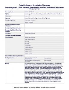
Knowledge discovery is an iterative process consisting of several steps including selection, preprocessing, transformation, data mining, and interpretation and evaluation [8]. We have worked collaboratively with the scientists at the Naval Oceanographic Office (NAVOCEANO) at the Stennis Space Center to develop a knowledge discovery process for extracting provinces of similar visual texture from a database of very large acoustic images using the unsupervised learning algorithm AutoClass [7]. This process is described in detail in Hodges et al. [9] and Bridges et al. [3] and is illustrated in figure 1. We first extract gray-level co-occurrence matrices using quantized (0..15) pixel values from regions in the image data. We then compute textural statistics on these gray level co-occurrence matrices to obtain a vector of features for each region [3, 10, 15]. We performed the data-mining step on this set of feature vectors using AutoClass to cluster the instances. Finally, we mapped the categorized regions back onto a copy of the original image by assigning a specific color or gray scale to each class and coloring the pixels in each region with the color associated with that region’s class. The clustering step within our data mining process required significantly more computational time than all the other steps in the process and requires all the training data to be resident in RAM during the training process. Our current image data consists of 16 images requiring approximately 220 Megabytes of disk space, but we expect to be working with over 300 image files requiring over 1.5 Gigabytes of storage in the near future. Accommodating massive amounts of data requires some scaling technique to be applied to the data-mining algorithm. The excessive time required to process the learning phase suggest the use of multiple processors. One approach to scaling the data mining process is to embed the scaling techniques directly in the learning algorithm. Two research groups have recently reported algorithms that accomplish this by performing incremental learning [2, 11]. An

alternative approach is to partition the data into subsets, distribute the subsets to different processors, apply a sequential learning algorithm on each subset, and combine the learned results into a single classifier[4].

A c o u s t ic Im age

R e g io n e x t r a c t io n

F e atu re e x t r a c t io n

G LCM d e s c r ip t io n o f t e x e ls

(I n st-1 a 1 b 1 c 1) (I n st-2 a 2 b 2 c 2) . . . . . . (I n st-n a n b n cn)

C la s s if ic a t io n

F e a tu r e v ec to r r e p r e s e n t a t io n o f in s t a n c e s

C la s s 1 In st- 1 In st- 4 5 In st- 7 7 C la s s 2 In st- 1 4 In st- 1 0 5 In st- 3 0 0

C la s s m ... T e xtu re c la s s e s

V is u a liz a t io n

C la s s if ie d Im ag e

Figure 1. The knowledge discovery process for provincing of the ocean floor

Almost all previous work on the latter approach has been done with supervised learning systems where the correct classification is identified in the training data. The process of combining output from the different base classifiers may be as simple as a majority voting rule, or may use all the training data on all the bases classifiers and use the results to train a meta-classifier [4]. This meta-classifier is then used to combine the results from base classifiers. Our domain, unsupervised learning, does not have the correct answer available to train this meta-categorizer. Additionally, a cluster called cluster X in one categorizer may not correspond to cluster X in another categorizer. Combining the results from multiple categorizers in unsupervised learning requires we match up the clusters by predicting on all categorizers using a subset of all the training data and correlating the results. In this paper we describe a method we have developed to extend the meta-learning approach of Chan and Stolfo [4, 5] to unsupervised learning. We also report some preliminary results obtained by using this method to categorize regions in our acoustical images of the ocean floor.

2.

Combining Categorizers For Unsupervised Learning

We have developed an approach for adapting Chan and Stolfo’s meta-learning techniques for use with unsupervised learning. One technique adapted, the use of an arbitration rule and arbiter, is presented in Wooley et al. [16]. The technique addressed in this paper is based on Chan and Stolfo’s meta-learning technique that uses a combiner [4] as shown in figure 2. This approach divides the data into P disjoint data sets and trains P base classifiers. The role of the combiner is to learn the relationship between the predictions made by the P independent base classifiers so it can produce an accurate final prediction. Chan and Stolfo [4] present two techniques for creating instances to be used in the meta-level training. The first technique is to include in each instance the predictions from each of the base classifiers as well as the correct classification. This first technique is referred to as class-combiner. The second technique is to start with instances as in the class-combiner, and add the attribute vector from the raw data that was used to train the base classifiers. This second technique is referred to as class-attribute-combiner. Adapting Chan and Stolfo’s technique to unsupervised learning requires that the combiner learn how to associate the category relationships as well as conflicts that arise by inconsistent predictions from the base categorizers. The technique we used for this paper corresponds to Chan and Stolfo’s class-combiner, which uses the output of all the base categorizers to generate a new set of feature vectors. These feature vectors are then used to train an unsupervised learning algorithm that performs the function of the combiner. The training phase divides all the training instances (I1 . . Ix) into P disjoint data sets (D1 . . DP), which are then distributed to the P processors and used to train the P independent categorizers (C1 .. CP). Each categorizer identifies a certain number of categories in the data. The jth category of categorizer Ci is referred to as cij. A subset of the instances (Ik) is then selected so that there are instances from all the Dp. Each of these Ik is processed by all P categorizers producing a new feature vector FIk = {c1j, c2j’, c3j’’, … cPj’’’’} for each Ik. To complete the meta-training, this new set of feature vectors are trained using an unsupervised learning algorithm (AutoClass) to produce a new set of categories (N1 .. NL). To use this system in prediction mode, an instance Ik is submitted to each of the base categorizers resulting in a new feature vector FIk = { c1j, c2j’, c3j’’, … cPj’’’’}. This feature vector is submitted to the combiner which predicts which category it belongs in (N1 .. NL), which is the final categorization of the instance Ik. As the number of processors (P) increase, the size of the feature vector also increases. The training time required for meta learning is significantly less than for the original categorizers. This is because the new feature vector contains a smaller number of features, the features are nominal data, there is a large amount of duplication in the feature vectors, and each feature has restrictions on the range imposed by the maximum number of classes in each base categorizer.

C la s s ifie r 1

P r e d ic tio n 1

I n s ta n c e

C o m b in e r

C la s s if ie r 2

P r e d ic tio n 2

Figure 2. An arbiter with two classifiers. From [4].

3.

The Classification Task And Data

The categorization system we are working with uses the visual texture of acoustic images to “province” the ocean floor. The acoustic images (provided by NAVOCEANO at Stennis Space Center) were collected from a 100 kHz Chirp SideScan Sonar using a Data Sonics SIS1000. Figure 3a gives an example of a portion of one of these images. A region-growing process based on the techniques described in Reed and Hussong [13] is used to divide each image into irregularly shaped homogeneous regions that are the instances to be categorized. A more detailed description of our implementation of region-growing is provided in Wooley and Smith[15] and Bridges et al.[3]. Four gray-level co-occurrence matrices (GLCMs) are computed for each region (one in each of 4 directions). Secondary texture statistics are computed from the GLCMs as described in Bridges et al.[3] and Karpovich [10]. These statistics are used to form a feature vector for each region (instance). AutoClass C was obtained from NASA Ames[12] and used to cluster the images. Categorized images are built, which correspond to the original images, and the results of the knowledge discovery process are evaluated visually.

4.

The Parallel Processing Environment

Our objectives in designing the parallel environment for clustering algorithms were twofold. First, we wanted to make minimal (or no) changes to the source code of the clustering algorithms. Second, we wanted the ability to run each process of a parallel clustering algorithm execution on a different dataset in both the learning and classification modes. Additionally, we used the Message Passing Interface (MPI) library[14], a de facto standard for parallel processing, to write our parallel programs, making our system executable in a wide variety of parallel environments. Much of the parallelization effort involved writing the programs to distribute data and gather results along with some changes to the clustering algorithm. Although changes were made to the clustering algorithm (AutoClass) for this parallelization

process, we are developing a parallel shell that will allow the use of any clustering algorithm without changes. The serial (original) version of AutoClass reads and creates files with fixed names, which is problematic since we run several instances of AutoClass simultaneously. In order to eliminate the analysis and code modification required to make each AutoClass process use files with unique names, we wrote a few lines of MPI code to change the working directory of each AutoClass process, based on its process index. This allows each process to execute in its own area, without possibility of file name collisions. The hardware we used for our experiments was an Avalon A12 multicomputer consisting of eight DEC Alpha 21164A CPUs running at 400MHz [1]. Each processor on this distributed memory machine has 256 megabytes of RAM. Interprocessor communication is provided via a fully interconnected 14-channel crossbar switch, with each channel supporting data-streams of 400 megabytes per second, or 200 megabytes per second in each direction.

5.

EXPERIMENTS AND RESULTS

In the experiments described below, the data (feature vectors) were extracted from 12 acoustical images that were split into two parts to eliminate the shiptrack. Since there is no known “correct” class for each of the instances, the classification results from the multicomputer runs were visually compared to those from the single processor run. Results from single processor runs were evaluated based on information provided by geologists at NAVOCEANO. The algorithm described above was run on 1 to 8 processors. Instances from the training dataset were distributed to the processors. We fixed the number of classes at 9, which generated good results for single processor experiments performed in the past. The training time for the distributed training data is linear as expected, and the training time for the meta-learning using 20% of the original data is relatively constant, and significantly less than the training time of a base categorizer on 20% of the data. This is due to the reduced number of features, the nominal data types in the feature vectors, and to the large amount of duplication in the feature vectors. The results of prediction for each of the different number of processors are shown for an example image in figure 3. Figure 3 contains six images. The first image (figure 3a) is the original sonar image of the ocean floor. The other five images are resultant images after applying clustering algorithms to categorize the regions of the original image. The label on each of the classified images identifies the number of processors (e.g. P3 – three processors) that participated in the clustering process. The gray scale shade of each image is insignificant. What is important is the patterns identified by the shading and how closely they represent the similar texture regions in the original image. Note that the patterns from all the images are similar. These initial results are very encouraging. We are in the process of refining this technique and of developing more objective means of evaluating the results.

6.

ACKNOWLEDGEMENTS

This work was sponsored by the Office of Naval Research under grant ONR-N0001496-1276, by Mississippi State University College of Engineering from the Hearin Educational Enhancement Fund, and NASA Stennis under grant NAS1398033-2099010033.

References 1.

Avalon Computer Systems, Inc. 1998. Avalon Series A12 Parallel Supercomputers. http://www.teraflop.com/html/a12.html, accessed May 15, 1998.

2.

Bradley, P. S., Usama Fayyad, and Cory Reina. 1998. Scaling clustering algorithms to large databases. In Proceedings of the Fourth International Conference on Knowledge Discovery and Data Mining. Edited by Rakesh Agrawal and Paul Stolorz. Menlo Park, CA: AAAI Press. 9-15.

3.

Bridges, Susan, Julia Hodges, Bruce Wooley, Donald Karpovich, George Brannon Smith. 1998. Knowledge discovery in an oceanographic database. Submitted for publication.

4.

Chan, Philip K., and Salvatore J. Stolfo. 1995. Learning arbiter and combiner trees from partitioned data for scaling machine learning. In Proceedings of the First International Conference on Knowledge Discovery and Data Mining. Edited by Usama Fayyad and Ramasamy Uthurusamy. Menlo Park, CA: AAAI Press. 39-44.

5.

Chan, Philip K., and Salvatore J. Stolfo. 1996. Scalable exploratory data mining of distributed geoscientific data. In Proceedings of the Second International Conference on Knowledge Discovery and Data Mining. Edited by Evangelos Simoudis, Jiawei Han and Usama Fayyad. Menlo Park, CA: AAAI Press. 2-7.

6.

Cheeseman, Peter, and John Stutz. 1996. Bayesian classification (AutoClass): Theory and results. Advances in Knowledge Discovery and Data Mining. Edited by Usama M. Fayyad, Gregory Piatetsky-Shapiro, Padhraic Smyth, and Ramasamy Uthurusamy. Menlo Park, CA: AAAI Press. 158-180.

7.

Cheeseman, P. J. Kelly, M. Self, J. Stutz, W. Taylor, and D. Freeman. 1988. AutoClass: A Bayesian classification system. In Proceedings of the Fifth International Conference on Machine Learning. Reprinted in Readings in Machine Learning, edited by Jude W. Shavlik and Thomas G. Dietterich, San Mateo, CA: Morgan Kaufmanns Publishers, Inc. 296-306.

8

Fayyad, Usama M., Gregory Piatetsky-Shapiro, and Padhraic Smyth. 1996. From data mining to knowledge discovery: An overview. Advances in knowledge discovery and data mining. Edited by Usama M. Fayyad, Gregory Piatetsky-Shapiro, Padhraic Smyth, and Ramasamy Uthurusamy. Menlo Park, CA: AAAI Press. 1-36.

9.

Hodges, Julia, Susan Bridges, Bruce Wooley, Donald Karpovich, and Brannon Smith. 1997. Knowledge Discovery in an Object-Oriented Oceanographic Database System. October 21, 1997. Mississippi State University Technical Report #971021.

10. Karpovich, Donald. 1998. Choosing the optimal features and texel sizes in image categorization. In Proceedings of the 36th ACM Southeast Conference held in Marietta, GA, April 1-3, 1998. 104-107 11. Livny, Miron, Raghu Ramakrishnan, and Tian Zhang. 1998. Fast density and probability estimation using CF-Kernel method for very large databases. http://www.cs.wisc.edu/~zhang/birch.html, accessed Oct 1998. 12. NASA Ames Research Center, Computational Sciences Division. 1998. AutoClass C General Information. http://ic-www.arc.nasa.gov/ic/projects/bayesgroup/autoclass/autoclass-c-program.html, accessed May 15, 1998. 13. Reed, Thomas Beckett IV, and Donald Hussong. 1989. Digital image processing techniques for enhancement and classification of SeaMARC II side scan sonar imagery. Journal of Geophysical Research. 94(B6). 7469-7490. 14. Snir, Marc, Steve W. Otto, Steven Huss-Lederman, David W. Walker, and Jack Dongarra. 1996. MPI: The Complete Reference. Cambridge, Massachusetts: The MIT Press. 15. Wooley, Bruce and George Brannon Smith. 1998. Region-growing techniques based on texture for provincing the ocean floor. In Proceedings of the 36th ACM Southeast Conference held in Marietta, GA, April 1-3, 1998. 99-103. 16. Wooley, Bruce, Yoginder Dandass, Susan Bridges, Julia Hodges, And Anthony Skjellum. 1998. Scalable knowledge discovery from oceanographic data. In Intelligent engineering systems through artificial neural networks. Volume 8 (ANNIE 98). Edited by Cihan H Dagli, Metin Akay, Anna L Buczak, Okan Ersoy, and Benito R. Fernandez. New York, NY: ASME Press. 413-24.

(a)

P1

P5

P7

P3

P8

FIGURE 3. Comparison of images trained with p processors