Ecological Modelling 222 (2011) 3011–3019
Contents lists available at ScienceDirect
Ecological Modelling journal homepage: www.elsevier.com/locate/ecolmodel
Scaling-up spatially-explicit ecological models using graphics processors Johan van de Koppel a,∗ , Rohit Gupta a,b , Cornelis Vuik b a b
Spatial Ecology Department, The Netherlands Institute of Ecology (NIOO-KNAW), Post Office Box 140, 4400 AC Yerseke, The Netherlands Delft University of Technology, Faculty EEMCS, Delft Institute of Applied Mathematics, 07.060, Mekelweg 4, 2628 CD, Delft, The Netherlands
a r t i c l e
i n f o
Article history: Received 7 September 2010 Received in revised form 24 April 2011 Accepted 6 June 2011 Available online 19 July 2011 Keywords: CUDA Graphics processors Scaling laws Self-organization Spatially explicit models
a b s t r a c t How the properties of ecosystems relate to spatial scale is a prominent topic in current ecosystem research. Despite this, spatially explicit models typically include only a limited range of spatial scales, mostly because of computing limitations. Here, we describe the use of graphics processors to efficiently solve spatially explicit ecological models at large spatial scale using the CUDA language extension. We explain this technique by implementing three classical models of spatial self-organization in ecology: a spiral-wave forming predator–prey model, a model of pattern formation in arid vegetation, and a model of disturbance in mussel beds on rocky shores. Using these models, we show that the solutions of models on large spatial grids can be obtained on graphics processors with up to two orders of magnitude reduction in simulation time relative to normal pc processors. This allows for efficient simulation of very large spatial grids, which is crucial for, for instance, the study of the effect of spatial heterogeneity on the formation of self-organized spatial patterns, thereby facilitating the comparison between theoretical results and empirical data. Finally, we show that large-scale spatial simulations are preferable over repetitions at smaller spatial scales in identifying the presence of scaling relations in spatially self-organized ecosystems. Hence, the study of scaling laws in ecology may benefit significantly from implementation of ecological models on graphics processors. © 2011 Elsevier B.V. All rights reserved.
1. Introduction In the past years, spatially-explicit mathematical models have played an important role in the development of ecological theory (Levin, 1992; Rohani et al., 1997; Rietkerk and Van de Koppel, 2008). They have been used to gain understanding of the importance of space in the dynamics and conservation of species in both continuous (Hassell et al., 1994; Solé and Bascompte, 2006) and fragmented habitats (Hanski, 1994; Gravel et al., 2010). Especially models of spatial self-organization have been used to implement complexity theory principles to ecological systems. These models have been applied to for instance, spatial wave formation in large-scale predator-prey systems (Dunbar, 1983), to explain the formation of regular, self-organized spatial patterns in arid vegetation (Klausmeier, 1999), and scale-free patterns in disturbance-governed rocky intertidal mussel beds (Guichard et al., 2003). The basic premise behind self-organization models is that small-scale interactions between organisms generate coherent spatial patterns at larger spatial scales (Levin, 1992). Predicted patterns involve regular banded, dotted or labyrinth-shaped patterns that have been observed in many ecosystems all over the world (Rietkerk and Van de Koppel, 2008), and “power law” pat-
∗ Corresponding author. Tel.: +31 113 577455. E-mail address:
[email protected] (J. van de Koppel). 0304-3800/$ – see front matter © 2011 Elsevier B.V. All rights reserved. doi:10.1016/j.ecolmodel.2011.06.004
terns that have universal characteristics over an extensive range of spatial scales, e.g., are scale-free (Pascual and Guichard, 2005). As theoretical models predict consistent changes in spatial patterns with changing environmental conditions, self-organized spatial patterns have been put forward as promising predictors of imminent degradation and desertification in ecosystems in response to global change (Rietkerk et al., 2004; Kefi et al., 2007b; Solé, 2007; Scheffer et al., 2009). Despite the common use of spatial models to scale-up the effects of ecological interactions, most spatially-explicit models cover only a limited range of spatial scales. Partial differential equations that form the basis for most models of regular patterns are typically implemented on rectangular grids of 100 × 100 to 250 × 250 nodes. This allows a basic, limited scale prediction of regular pattern formation, but does not allow for the analysis of patterns along intrinsic or imposed gradients, modeling of nested patterns, or inclusion of evolutionary dynamics (because of the time scale differences between ecological and evolutionary processes). Cellular automaton models can be implemented over larger scales, but rarely exceed a size of 500 × 500 nodes. Yet, accurate fits of power law-shaped size-frequency distributions to describe patch formation depend crucially on precise predictions of the frequency of occurrence of large clusters or patches, which are often limited by the size of the simulated grid. Hence, to provide accurate predictions of the response of spatially self-organized systems to changing conditions, and to assess the value of the predicted
3012
J. van de Koppel et al. / Ecological Modelling 222 (2011) 3011–3019
patterns for indicator systems, predictions over extensive spatial scales are essential. Here, we report on the use and implementation of graphics processors to efficiently solve spatially explicit ecological models on large spatial grids. Graphics processors, a common component of off-the-shelf multimedia computers, typically house a large number of processing cores that can efficiently process large grids, provided that the changes at each node (e.g., a point at the grid) can be predicted in parallel. This is the case for most spatial models where the entire grid is synchronously updated at the end of a single computing cycle (e.g., timestep). We describe how numerical algorithms are implemented on the graphics processor using the CUDA framework that is available for modern NVidia graphics cards. We provide example codes of implementations of three classical spatial models within ecological theory, the spiral-wave forming predator–prey model of Dunbar (1983), the model of selforganizing arid vegetation patterns by Rietkerk et al. (2002), and the mussel disturbance model by Guichard et al. (2003). We then study how the predictions of the models are affected by increased spatial scale. 2. Spatially explicit ecological models Most ecological models described in theoretical ecology textbooks describe the changes in populations and the environment at a particular spatial location, or average their density over a particular spatial scale (e.g., a mean-field approach). Implicitly, these models assume that the heterogeneity that exists in natural systems at nearly every spatial scale is not of major influence to population dynamics. For many systems and for many modeling goals, this assumption does not hold. In these cases, the spatial structure of the population and the spatial movement of organisms and matter need to be modeled explicitly. Examples of this are the spatial dynamics of disease outbreaks, or the formation of regular spatial patterns in arid lands, which are described using spatially explicit models. Spatially explicit models are often solved numerically using a spatial grid approach. At each node on the grid, both local population change and spatial fluxes are calculated as a function of population size at the node itself and the neighboring nodes (the scale of the neighborhood can be very local or more extensive). Often, the same calculations are repeated over the entire grid, calculating how population size at each node would change as described by a partial differential equation. In most modern computers, the rates of change are calculated for one node after the other until calculation has finished for the entire grid and population level at all nodes can subsequently be updated. A special type of spatial model is the cellular automaton, which describes the spatial structure of any population using discrete states at each node, for instance being an individual of a specific species of plant. A node can change in state, for instance an individual plant being replaced by another, in a stochastic process, in which the replacement chance is a function of the state of the neighboring nodes. Similar to the partial-differential equation-based models, the same numerical operation is done for each node on the grid, calculating the new states based on the occupancies of the nodes in its current state. 3. Solving spatially explicit ecological models using a graphics processor Normally, simulation models are executed by the computer’s central processing unit, or CPU. Nearly all computers that are sold these days, however, also contain a graphics processing unit, or GPU, that handles the rendering of graphics before they are dis-
played on the screen. GPUs are either integrated within the main board of the computer, or placed on dedicated graphics cards. In particular GPUs on graphics cards are often very powerful computing chips. Rather than being able to do a broad range of tasks, which is the domain of the CPU, GPUs are specialized in floating point operations, e.g., calculations with numbers with many decimals. Another characteristic of modern GPUs is that they contain multiple cores, allowing the GPU to do many calculations at the same time. While current CPUs in personal computers contain between a single to four cores, high-end GPUs nowadays can contain many hundreds of cores per GPU, and hence can do a very high number of floating point calculations at the same time. These characteristics make graphics cards particularly suited to numerically solve spatially explicit models, especially those that are based on the above-described grid approach. The rates of change in several nodes can be calculated in parallel, which will significantly speed up the simulation. The use of GPUs for parallel computation, for instance in solving spatially explicit ecological models, has to a large extent been limited by the difficulties of addressing them from mainstream computing languages such as C, Fortran or MatLab. Recently, GPU manufacturers are facilitating the use of graphics processors for custom programming applications by providing language extensions to standard programming languages. The mostly widely used extension at this moment is CUDA, the parallel computing architecture developed by NVidia for their GPUs. CUDA is an extension of C which can be used to execute the kernel of a simulation model (e.g., the part that gets repeated each time step) on the graphics processor. When a spatially explicit simulation model is implemented on the graphics processor, execution speed can increase between 10and 100-fold as compared to a standard C implementation on the main processor, depending on the type of graphics card, the size of the grid and the type of spatial model. Below, we first explain conceptually how a spatially explicit model is implemented on a graphics processor using CUDA. Then we provide three examples implementations of well-known spatially explicitly models from ecological theory to illustrate this technique, examples that can form an easy starting point for further model development. These example models are the predator–prey model by Dunbar (1983), the self-organizing arid vegetation model by Rietkerk et al. (2002), and the mussel bed disturbance model by Guichard et al. (2003). We briefly review these models, and then describe their implementation in CUDA. Note that the implementation of spatially explicit models on graphics processors, or in parallel processors in general, implies that all nodes are updated synchronously (e.g., at the same time). Asynchronous updating, where the nodes are updated in sequence (e.g., after each other), requires just a single thread, and is therefore best implemented on a single core, typically the CPU. 3.1. Implementing a spatially explicit model in CUDA To run a spatially explicit simulation model on the GPU, it is crucial to understand how parallel processing of a spatial model is organized (Fig. 1). The calculations required to predict the rate of change at any node are called a thread. Each thread is processed by a specific processor core which has its own local memory to be used in calculations within the thread. However, the grids used in spatial models can easily have over 10,000 gridpoints, and hence even with the most extensive GPUs, each core has to handle multiple threads before the entire grid is updated. Haphazardly assigning processing cores to threads would be very inefficient. For this reason, the grid is split up in blocks, which is handled by what is called a multiprocessor, a group of 8 processor cores. This block has its own “shared” memory in which the variables needed to process the threads within this block are copied. Hence, the grid values
J. van de Koppel et al. / Ecological Modelling 222 (2011) 3011–3019
3013
Thread Per-thread local memory
Thread Block
Per block shared memory
Grid 1 Block ( 0 , 0 )
Block ( 1 , 0 )
Block ( 2 , 0 )
Global memory Block ( 0 , 1 )
Block ( 1 , 1 )
Block ( 2 , 1 )
Fig. 1. Organization of computation and memory hierarchy on the GPU by the CUDA programming model. The computation of changes in the state of each node is called a thread. Threads are organized in blocks on which a multiprocessor operates, and all the thread blocks which make up the entire spatial grid. Each level has its own memory. See text for explanation.
used within this block are loaded into the multiprocessor’s shared memory, allowing it to efficiently process all threads without additional access to the global GPU memory outside the multiprocessor, on which the entire grid is stored. The block structure ensures that the transfer of data from the graphics card’s global memory to the graphics processor register memory is handled in an efficient way, preventing separate memory transfers for each individual thread. For best performance it is important that the information needed by each thread is local (e.g., from neighboring nodes), e.g., does not originate from the other side of the grid, so that it can all be loaded in the multiprocessor’s memory before the block is executed. When developing a model to run on the GPU, it is essential to optimize the size and number of the blocks, so that all processing cores are used efficiently. Obviously, a block size is limited by the size of the multiprocessor’s memory, and hence large block sizes are not optimal. Beyond that, it is essential that the number of blocks is adjusted to the number of multiprocessors. For instance, if a GPU has 6 multiprocessors (e.g., 48 cores), it is inefficient to split the grid up into 8 blocks. Six blocks would then be first processed, after which two blocks remain. These would subsequently be processed by two multiprocessors, leaving the others waiting until those two have finished. It would be more efficient to divide the grid into 12 smaller blocks, so that after two rounds, all blocks have been processed and no multiprocessors remained idle for part of the time. The number of multiprocessors and the size of their internal memory are specific to the type of GPU and graphics card; more expensive graphics cards have more multiprocessors and more memory. This means that in order to maximize the acceleration, the model needs to be geared to the GPU in the computer and recompiled before the model is run. However, a thread block size of 16 × 16 (256 threads) is a common choice that gave us good simulation results. More details about how to design an optimal configuration can be found in the NVidia CUDA programming guide at www.nvidia.com/cuda.
3.2. CUDA: an extension of the C language Within any model program, the code needs to indicate which part of the program needs to be executed on the graphics processor. For this, a C language extension is provided that indicates that certain parts of the code need to be executed on the GPU, and that variables (most notably the arrays containing the state values at each node) and constants (e.g., the model’s parameter values) need to be placed on the graphics processor before they are executed. For this, these variables have to be labeled specifically in the code using specific variable and function definitions that have been developed. This is best explained using an example code. For this, we use Fisher’s equation for a biological invasion of a species U in a spatial domain (Fisher, 1937): ∂U ∂2 U . = U(1 − U) + ∂t ∂x2 In this equation, local growth is modeled by the first term, the logistic growth equation with both intrinsic growth and maximum local density set to 1. Dispersal of organisms is modeled by the second term using a diffusion approximation. This model describes the formation of an invasion front that moves from one side of the domain to the other, starting with an initial condition where population density is one at the edge of the domain, and zero in the remaining space. We will describe the implementation of this model in CUDA below, assuming a basic understanding of the C programming language. In Table 1, an example code is given that implements Fisher’s equation along a one-dimensional domain U. This code describes how to implement the kernel that calculates the rate of change of local population density U in CUDA. For this, we need to copy the initial values of the domain U to the graphics processor, run the kernel that calculates the changes in U using the above equation for a number of times, and then copy the results back from the GPU memory to the CPU memory. We start with describing how the comput-
3014
J. van de Koppel et al. / Ecological Modelling 222 (2011) 3011–3019
Table 1 A condensed example of a CUDA program, implementing Fisher’s equation describing a biological invasion. 1 2 3 4 5 6 7 8 9 10 11 12 13 14 15 16 17 18 19 20 21 22 23 24 25 26 27 28 29 30 31 32 33 34 35 36 37 38 39 40 41 42 43 44 45 46 47 48 49 50 51 52 53 54 55 56 57 58 59
// includes, system & CUDA #include #include // Parameter definitions #define Block_Size 4 // Thread block size #define Block_Number 16 // Number of blocks in the grid #define Grid_Width (Block_Number*Block_Size) // Domain width #define Length 100 // The Length of the landscape #define dT 0.1 // Time step /* ------- Device function that calculates U flux-------*/ __device__ float d2Udx2(float* U, int current) { float dx, retval; dx=(float)Length/Grid_Width; retval = ( (-( U[current] - U[current-1] ) / dx ) -(-( U[current+1] - U[current] ) / dx ) ) / dx ; return retval;} /* ----------- Main Simulation Kernel ---------------------*/ __global__ void dUdt_Kernel (float* U) { int current; current = blockIdx.x*Block_Size+threadIdx.x; // The actual calculations for the model if (current > 0 && current < Grid_Width-1) { // excluding the boundaries U[current]=U[current]+(U[current]*(1-U[current])+d2Udx2(U,current))*dT; } __syncthreads(); } // End assembleMusselKernel /* ---------- Program main -----------------------------------*/ int main(int argc, char** argv){ unsigned int size_U = Grid_Width; unsigned int mem_size_U = sizeof(float) * size_U; float* h_U, * d_U; int time,x,i; FILE *fp; h_U = (float*) malloc(mem_size_U); // allocate host memory for(x=0;x