Simultaneous Batching and Scheduling Using Dynamic Decomposition on a Grid Michael C. Ferris Computer Sciences Department, University of Wisconsin – Madison 1210 West Dayton Street, Madison, WI, 53706, USA,
[email protected]
Arul Sundaramoorthy, Christos T. Maravelias Department of Chemical and Biological Engineering, University of Wisconsin – Madison 1415 Engineering Dr., Madison, WI 53506, USA {
[email protected],
[email protected]}
Scheduling problems arise in many applications in process industries. However, despite various efforts to develop efficient scheduling methods, current approaches cannot be used to solve instances of industrial importance in reasonable time frames. The goal of this paper is the development of a dynamic decomposition scheme that exploits the structure of the problem and is well suited for grid computing. The problem we study is the simultaneous batching and scheduling of multi-stage batch processes. The algorithm first decomposes the original problem into 1st-level subproblems based on batching decisions. The subproblems that remain unsolved within a resource limit are then dynamically decomposed into 2nd-level subproblems based on batch-unit assignment decisions in one stage. The process can be repeated in a dynamic fashion by identifying subproblems that cannot be solved within a given resource limit and decomposing them by batch-unit assignment, until all subproblems are solved. Alternatively, a problem can be decomposed into a number of promising subproblems using an automatic strong branching scheme. Our results show that the proposed method can be used on a grid computer to solve large problems to optimality in reasonable computational time. Keywords: Chemical batch processes; batching and scheduling; mixed-integer programming; grid computing; decomposition algorithm.
1. Introduction Production scheduling is a very important and challenging problem in many process industries. For example, in the petroleum sector, scheduling problems arise in the transportation and unloading of crude oil from pipelines, the transfer to storage tanks and the charge for each crude oil distillation unit. In basic chemical and consumer products, scheduling problems typically involve the sequence of production in continuous processing units, while in the pharmaceutical and specialty chemical sectors, scheduling problems involve the allocation of limited resources (e.g. processing and storage units) to competing products and the sequencing of batches on units. In terms of plant configurations, the most common structure of batch processes is the multi-stage multi-product batch structure, where a number of products compete for a set of limited resources, each product has to be sequentially processed in a number of stages, and each stage contains one or more parallel processing units (see Figure 1). Batch splitting and mixing are not typically allowed and there are no recycle streams. Note that the flow-shop and multiple-unit (or single-stage) problems can be viewed as special cases of the multi-stage problem (Pinedo 2002). Further, different storage policies such as limited/unlimited/no intermediate storage and transfer policies can be employed based on the nature of products and the availability of resources. The scheduling of multi-stage batch processes has received significant attention from researchers in the process systems engineering community (see Pinto and Grossmann, 1998; Pekny and Reklaitis, 1998; Shah, 1998; and Méndez et al., 2006 for reviews). Existing methods assume that batching and scheduling decisions are made independently, i.e. each order is divided into a number of batches (batching), which are then assigned to processing units and sequenced (scheduling). For the sequencing of batches there exist two different approaches: i) slot-based (Pinto and Grossmann 1996, Lamba and Karimi 2002) and ii) sequence-based (Hui and Gupta, 2000; Mendez et al., 2001; Gupta and Karimi, 2003). To address larger instances, several researchers have developed decomposition techniques. Harjunkoski and Grossmann (2002), Maravelias and Grossmann (2004) and Roe et al. (2005) developed hybrid methods that use mixed-integer programming (MIP) and constraint programming (CP) techniques. Maravelias (2006) presented a decomposition technique that combines MIP and problem-specific algorithms. Finally, Neumann et al. (2002) and Kelly (2002, 2003) developed MIP-based decomposition algorithms (see Mendez et al. (2006) for a review of the most widely used decomposition techniques). Finally, Prasad and Maravelias (2007) developed a MIP formulation for the simultaneous batching and scheduling of multi-stage batch processes. Their formulation was shown to yield better solutions than previous sequential approaches, where batching is carried out independently from scheduling. Although the time horizon of scheduling problems in the chemical industry typically varies between one week and one month, a process facility may be re-scheduled on a daily basis. This is because new orders with tight deadlines often have to be inserted in existing schedules, release dates have to be updated due to delays in raw material deliveries, and processing delays and equipment failures cause major disruptions. Therefore, the development of solution methods that allow us to solve real-world
2
problems in a few hours is imperative. However, despite the advances in computer hardware and optimization software, existing approaches are insufficient to address real world problems. Batch scheduling, specifically, remains a notoriously hard problem. The subject of this paper is the development of a dynamic decomposition algorithm that can harness the computational resources of grid computing and the Condor management system, enabling us to solve large scheduling problems. Our goal is to show that if problem-specific knowledge is used to develop a solution method that exploits modern computing tools, then rigorous mathematical programming models can be can be solved in reasonable wall clock time and thus used for practical decision making. In this paper we study the MIP formulation of Prasad and Maravelias (2007) because it is a MIP formulation that can be used to address a wide range of problems in multi-stage batch processes, but it is also one of the hardest MIP models for batch scheduling. However, we believe that the major ideas behind the method developed in this paper can be applied to other process optimization problems. The rest of the paper is structured as follows. In section 2, we formally define the problem at hand and present the MIP formulation for the simultaneous batching and scheduling in multi-stage batch processes. In section 3, we briefly discuss grid computing and in section 4 we present the proposed dynamic decomposition algorithm. Section 5 outlines our computational results on a number of prototypical examples of these problems and includes recommendations on how to utilize the grid computer most effectively. The paper concludes with a summary and some topics for further research.
2. Batching and Scheduling of Multi-stage Batch Processes 2.1. Problem Statement The problem of simultaneous batching and scheduling can be expressed as follows (see also Figure 1): Given (i)
a set of orders (i∈I) with release/due time ri,/di and demand qi,
(ii)
a set of processing units (j∈J) with minimum/maximum batch sizes bjmin/bjmax, and processing time
τij and processing cost cij for order i, (iii) a set of stages (k∈K) with parallel processing units (j∈J(k); J = J(1) ∪ J(2) …∪ J(|K|)) at each stage k, (iv)
a set of forbidden units FJ(i) for order i and a set of forbidden production paths (j,j′)∈FP for all orders,
determine (i) the number and size of batches required to meet each order (batching decision), (ii) the assignment of batches to processing units at each stage, (iii) the sequencing of assigned batches in each processing unit, in order to minimize the time necessary to meet all orders.
3
Orders: i ∈ I = {A, B, C}
Stages: k ∈ K = {1, 2, 3}
Batches
Units: j ∈ J = J(1) ∪ J(2) ∪ J(3)
qi rA
dA rB
rC
U3
A
dB dC
U1
U6 U4
B U2
C
U7 U5
k=1
k=2
k=3
J(1) = {U1, U2} J(2) = {U3, U4, U5} J(3) = {U6, U7}
Figure 1: Example of a multi-stage batch plant. It is assumed that all orders go through all stages, that unlimited storage is available for intermediates between stages, and that changeover times are negligible.
2.2. MIP Formulation To account for batching decisions, we first have to calculate the minimum (lmini) and maximum (lmaxi) possible number of batches that order i∈I can be divided to:
⎡q ⎤ lmini = ⎢ i ˆ max ⎥ ⎢ bi ⎥
∀i ∈ I
(1)
⎡q ⎤ lmaxi = ⎢ i ~ max ⎥ ⎢ bi ⎥
∀i ∈ I
(2)
where
(
bˆimax = min ⎡ max b max k∈K ⎢ ⎣ j∈JA ( i ,k ) j
(
)⎤⎥⎦ is
the
maximum
feasible
batch
size
for
order
i,
)
~ ⎤ is the largest batch size for order i that can be processed on all allowed units, bi max = min ⎡ min b max k∈K ⎢ ⎣ j∈JA (i ,k ) j ⎥⎦ and JA(i,k) = J(k)\FJ(i) is the set of units that can be used for the processing of order i in stage k (see Prasad and Maravelias (2007) for details). Once we have calculated lmaxi, we postulate a set L(i) = {1, 2, …lmaxi} of potential batches for each order i∈I. Thus, a batch is denoted by a pair (i,l): index i denotes the order that a batch corresponds to and index l∈L(i) denotes the batch number. The three major decisions for the simultaneous batching and scheduling of multi-stage process are modeled as follows: (i) Batch selection: Zil = 1 if the lth potential batch is active (i.e. selected to satisfy order i) (ii) Batch assignment: Xilj = 1 if batch (i,l) is assigned to processing unit j
4
(iii) Batch sequencing: Yili’l’k = 1 if batch (i’,l’) is processed after (i,l) on the same unit of stage k. The set of batches (i,l) and (i′,l′) that can be sequenced on a unit is denoted by IL:
IL = {i, i '∈ I , l ≤ lmaxi , l ' ≤ lmaxi : (i ≠ i ') ∨ ((i = i ') ∧ (l ≠ l '))} To reduce the number of symmetric solutions, the selection of batches is carried out in numerical sequence:
Z il ≤ Z i ,l −1
∀i ∈ I ,1 < l ≤ lmaxi
(3)
Obviously, the size Bil of batch (i,l) can be nonzero only if the corresponding binary Zil is active,
Bil ≤ bˆimax Z il
∀i ∈ I , l ≤ lmaxi
(4)
A selected batch must be processed exactly once on each stage,
∑X
j∈JA ( i ,k )
ilj
= Z il
∀i ∈ I , l ≤ lmaxi , k ∈ K
(5)
For each order i, the batch-sizes of the selected batches must satisfy the demand for order i:
∑B
l ≤lmaxi
il
≥ qi
∀i ∈ I
(6)
At any stage, the size Bil of batch (i,l) should be within the minimum and maximum capacities of the processing units where batch (i,l) is processed,
∑b
min j j∈JA ( i , k )
X ilj ≤ Bil ≤
∑b
max j j∈JA ( i ,k )
X ilj
∀i ∈ I , l ≤ lmaxi , k ∈ K
(7)
A sequence between batches (i,l) and (i’,l’) is enforced via (8) when both batches are assigned on the same unit in stage k:
X ilj + X i 'l ' j − 1 ≤ Yili ' l ' k + Yi 'l ' ilk
∀ ( i, l , i ' l ' ) ∈ IL : i ≤ i ', k ∈ K , j ∈ JA(i, k ) ∩ JA(i ', k )
(8)
If batch (i′,l′) is processed after batch (i,l), then (9) enforces the corresponding time delay,
Ti 'l ' k ≥ Tilk +
∑
j∈JA ( i ', k )
τi'j X i 'l ' j − M (1 − Yili 'l ' k ) ∀ ( i, l , i ' l ') ∈ IL, k ∈ K
(9)
where Tilk is the finish time of batch (i,l) at stage k. Also, a batch can be processed at stage k only after it is finished at stage k-1:
Ti ,l ,k ≥ Tilk −1 +
∑
j∈JA ( i , k )
τij X ilj
∀i ∈ I , l ≤ lmaxi , k ∈ K
(10)
Release and due time constraints are enforced via (11) (for k = 1) and (12) (for k = |K|), respectively. In addition, (11) and (12) provide a valid lower and upper bound for Tilk:
5
Tilk ≥ ri Z il + ∑
∑τ
ij k '≤k j∈JA ( k ',i )
Tilk ≤ d i Z il − ∑
∑τ
∀i ∈ I , l ≤ lmaxi , k ∈ K
X ilj
ij k '> k j∈JA ( k ',i )
X ilj
∀i ∈ I , l ≤ lmaxi , k ∈ K
(11) (12)
By enforcing that the sum of the processing times of the batches assigned to a unit must not exceed the time window available for processing, (13) excludes a number of infeasible assignments.
∑ ∑τ
i∈IA( j ) l ≤lmaxi
ij
⎧ ⎫ ⎧ ⎫ X ijl ≤ MS − min ⎨∑ min ( τ ij' )⎬ − min ⎨ri + ∑ min ( τ ij ' )⎬ ∀k ∈ K , j ∈ J (k ) i∈IA( j ) j '∈J ( k ') k '< k ⎩k '>k j '∈J ( k ') ⎭ i∈IA( j ) ⎩ ⎭
(13)
where IA(j)=I\FI(J) is the set of orders that can be assigned to unit j. Forbidden paths and forbidden assignments are enforced via (14) and (15), respectively.
X ilj + X ilj ' ≤ Z il X ilj = 0
∀i ∈ I , l ≤ lmaxi , ( j , j ' ) ∈ FP ∀i ∈ I , l ≤ lmaxi , j ∈ FJ (i )
(14) (15)
Clearly, at least lmini batches are required to meet the demand for order i. Since the selection of batches is carried out in sequence via (3), binaries Zil are fixed to 1 for l≤lmini:
Z il = 1
∀i ∈ I , l ≤ lmini
(16)
To reduce the size of the branch and bound tree, we avoid symmetric solutions by adding the following constraint,
Bil ≤ Bi ,l −1
∀i ∈ I ,1 < l ≤ lmaxi
(17)
Obviously, batches (i,l) with l>lmaxi cannot be selected, assigned and sequenced
Z il , X ilj , Bil , Tilk = 0 Yili 'l 'k = 0
∀i ∈ I , l > lmaxi , j ∈ J , k ∈ K
∀(i, l , i ' l ') ∉ IL, k ∈ K
Z il , X ilj , Yili 'l 'k ∈ {0,1}
Bil , Tilk ≥ 0
(18) (19)
In this paper, we are interested in the minimization of makespan, the objective function that leads to the hardest MIP models:
min MS
(20)
where the makespan MS must be greater than the finish time of all batches at the last stage,
MS ≥ Til|K |
∀i ∈ I , l ≤ lmaxi
(21)
The MIP model P we study in this paper consists of (3) – (21). We would like to stress here that for a given batch facility (i.e. fixed set K of stages and fixed set J of processing units) the size of model P
6
depends on the number of orders and the number of batches. Note that all variables and most constraints are defined over i∈I, and l≤lmaxi.. Therefore, for a set of orders the demand amount qi implicitly determines the size of the formulation via the calculation of lmaxi (see (2)).. Model P can be used to addresses a wide range of problems (e.g. maximization of production over a fixed time horizon, minimization of lateness/makespan) and it was shown to yield better solutions than existing methods. The introduction of additional decision variables, however, resulted in an increase in the size and complexity of the formulation. To enhance its solution, Prasad and Maravelias (2007) presented a preprocessing algorithm that exploits time window information to fix some sequencing variables and a class of tightening inequalities. Nevertheless, model P, as most MIP models for process scheduling, cannot be currently used for the solution of practical instances within a few hours of wall clock time.
3. Grid Computing We have implemented our solution approach for this problem within GAMS utilizing the grid options that are described in Bussieck et al. (2007). A model of computation that is very useful for optimization applications is the master-worker paradigm, and this is the model we adopt. The master processor runs a GAMS process that creates and spawns all the tasks, and also collects the results of each task. When using GAMS/grid, each task is created in a separate directory by the master process. The master process spawns the task for execution on a worker, and the existence of a file “finished” in the task directory signifies that the task has been completed. While writing a solution file might take a long time, creating the “finished” file can be done essentially instantaneously. A new task is created (by a script) each time GAMS encounters a solve statement in the model file. The existence of the “finished” file and the loading of the solution can be carried out within GAMS using the “handlecollect” primitive. This simple design means that the GAMS/grid mechanism can run with a variety of grid engines since the aforementioned script can be easily tailored for a specific grid engine. Furthermore, the grid extensions are part of the standard GAMS modeling language and thus available for use in any model written in this language. The particular grid engine that we use is provided by the Condor resource manager (Epema et al., 1996; Litzkow et al., 1988), and involves a large collection of machines all running the Linux operating system. Our implementation does not require that the workers share a file system with the master since this would significantly restrict the number of workers that could be used. Instead, the task directory is shipped by Condor to a “sandbox” on the worker machine in which the task is executed. Only the files whose timestamp has been updated are shipped back to the submitting machine. All of these details are hidden from the modeler; they are carried out automatically when the solve statement is encountered following a single line directive in GAMS to use the grid option:
7
modname.solvelink = 3; solve modname using mip minimizing z; Further examples of the GAMS syntax used for grid submission, and the underlying methods to deal with different grid engines can be found in Bussieck et al. (2007). It is important for efficiency of the computation to allow the master to pass updated information to a worker that is currently executing a task. For example, the master might become aware of a new incumbent value when processing a large branch and bound tree in parallel. GAMS/CPLEX allows an existing set of options to be updated in an executing optimization using a file trigger mechanism; whenever the executing CPLEX process sees a trigger file, it removes the trigger file, and reads and processes a new option file (this is similar to the interrupt mechanism that allows options to be interactively updated for a running solution process). However, in our case, the CPLEX process is running in a “sandbox” on the worker machine, and the master process is only able to create files in the original “task directory”. Our implementation overcomes this problem using a utility called “condor_chirp”. The program “condor_chirp” has three options: fetch, remove and put. Instead of just running a CPLEX process on the worker, an additional helper process also executes on the worker that repeatedly calls condor_chirp. The helper process runs continually in a loop checking periodically for the existence of the trigger file on the master (using fetch) and copies over the new option file if the trigger file exists. (Note that the trigger file on the master is removed by condor_chirp before the option file is fetched to avoid race conditions.) The helper process also puts newly found incumbent solutions (dumped out from the running CPLEX process using the GAMS/BCH facility) from the worker into the master copy of the task directory. The master process can monitor these files to see if the new incumbent from a worker is better than its current incumbent. In this way, the master GAMS process becomes aware of good solutions much sooner than if it were to wait for the completion of the worker task. Note that the helper process and condor_chirp are not needed if the master and worker processes share a file system. These utilities just enable us to mimic the functionality that our optimization method needs from such a shared file system. However, since we do not require our workers to share a file system, the number of workers that we can typically use at any given time is significantly more than 1000. Even though this is a computational resource shared by a community of users, we can typically sustain the services of over 600 workers for long periods of time. It is possible to use heterogeneous machines as workers, and we have implemented this for scheme for a grid consisting of Solaris, Windows and Linux machines. However in the results given here all workers used the same operating system.
8
4. Decomposition Algorithm The goal of the solution method described in this section is the sequential dynamic decomposition of problem P into subproblems of different levels of complexity. First, model P is decomposed into a set of 1st-level subproblems, where each subproblem has a fixed number of batches. Second, if a 1st-level subproblem remains unsolved after a predetermined resource limit is reached, it is decomposed into a set of 2nd-level subproblems with the unit-batch assignments fixed for all batches at a given stage. If a 2ndlevel subproblem is not solved within the given resource limit, then it is further decomposed into a set of 3rd-level subproblems, based on the assignment of batches at a second stage. The process can be repeated until problem P is decomposed into subproblems that can be easily solved or pruned. Each subproblem is a task created by the master process and spawned for execution on a worker. The details of the algorithm are presented in the next two subsections, while a schematic diagram of the algorithm is given in Figure 2. A pseudo-code is presented in Appendix A. An illustrative example of the decomposition algorithm is presented in Appendix B. P
Fixing Zil
P1
2 1
P
P2
P22
P3
PM2 2(2)
P32
Promising
Π1 = {P1, P2,…. PM}
PM1
P4
4 1
P
Π2 =
U Π2
m
, m = 1,2,….M
m
where, Π 2m = {P1m , P2m , P3m ,.....}
Non-promising
Fixing Xilj 4 1,1
P
4 1,2
P
4 1,3
P
4 1,M3(4)
P
Π3 = U Π 3sm , m = 1,2,….M m,s
s = 1,2,….
m m m m where, Π3s = {Ps,1 , Ps,2 , Ps,3 ,.....}
Promising
Non-promising
Figure 2: Schematic Diagram of the Decomposition Algorithm. 4.1. Fixing the number of batches At the first level, model P is replaced by a set Π1 of M1 subproblems {P1, P2, …, PM1}. Each subproblem Pm∈Π1 has fixed number of batches, i.e. it corresponds to a unique batching solution. Thus, if lim is the number of batches for order i∈I in a batching solution, then subproblem Pm corresponds to a combination {lAm, lBm, …} of batches with lmini ≤ lim ≤ lmaxi, ∀i∈I. Each 1st-level subproblem is generated by setting,
lmin i = lmax i = l im , ∀i ∈ I
(22)
in equations (3) – (21) of model P.
9
Note that if (22) is true, then all Zil variables are fixed via (16) and (18). Therefore, each 1st-level subproblem corresponds to a multi-stage scheduling problem with assignment and sequencing decisions only. The number of 1st-level subproblems is M 1 = in subproblem Pm is N m =
∑l
m i i
∏ (1 + l max − l min ) and the number of batches i
i
i
. In our implementation we spawn all M1 problems with a short time
limit since we observe that nearly all of these models are essentially easy to solve, and only one or two of them create difficulties for the solver. Furthermore, fixing the Z variables allows some simplifications in the model remaining to be processed.
4.2. Fixing batch-unit assignments While most of the 1st-level subproblems are either infeasible or pruned within a minute, a few of them cannot be solved to optimality within the given resource limit. These subproblems are decomposed into 2nd-level subproblems. Specifically, each hard subproblem Pm is decomposed into a set Π2m = {P1m, P2m, …, PM2(m)m} of M2(m) 2nd-level subproblems (note that the superscript denotes the parent subproblem). The decomposition at this level is based on the assignment of batches to units in a single stage kF. In this paper, we use the assignments in the bottleneck stage, i.e. the stage with the largest ratio of average processing times over number of processing times. The goal here is two-fold: a) Identify a subset of batch-unit assignments in stage kF that can potentially lead to good solutions. For each such promising assignment we generate a 2nd-level subproblem. b) Identify subsets of assignments that are not likely to lead to good solutions (non- promising assignments). For each such subset, we generate a single subproblem. A batch-unit assignment at stage kF is considered promising if it is balanced, i.e. if batches are evenly assigned across all units in J(kF). The rational behind this criterion is that in a minimum makespan schedule all the units of the bottleneck stage should be evenly loaded. If this is not the case, then a better solution can be obtained by moving some batches from a heavily loaded unit to a less heavily loaded unit. If fractional assignments were allowed, then a perfectly balanced assignment would be one where Nm/|J(kF)| batches are assigned to each unit in stage kF. Since fractional assignments are infeasible and near balanced assignments can result in good solutions, we consider a larger subset of promising m m assignments. Specifically, we calculate the minimum NJ MIN and maximum NJ MAX number of batches
that can be assigned to a single unit in stage kF:
⎢ Nm ⎥ NJ mMIN = ⎢α MIN ⎥ | J(k F ) | ⎦ ⎣
(23)
⎡ Nm ⎤ NJ mMAX = ⎢α MAX ⎥ | J(k F ) | ⎥ ⎢
(24)
where αMIN∈[0.8, 1] and αMAX∈[1.0, 1.2] (in this paper we use αMIN=0.9 and αMAX = 1.1).
10
m m Assignments where all units in stage kF have between NJ MIN and NJ MAX assigned batches are considered m m promising. Assignments where at least one of the units has less than NJ MIN or more than NJ MAX
assigned batches are considered non-promising. Each promising assignment is studied independently, i.e. a 2nd-level subproblem is generated by adding the following constraint in the formulation of the parent 1stlevel subproblem:
X ilj = 1, ∀j ∈ J (k F ), (i, l ) ∈ D( j )
(25)
where D(j) is the set of batches that are assigned to unit j in the current 2nd-level subproblem. All assignments that are due to a lightly (or heavily) loaded unit are considered simultaneously, i.e. a single 2nd-level subproblem is generated for each such subset of assignments by adding either (26) or (27) for a single unit in stage kF:
∑X
ilj
≤ NJ mMIN − 1
(26)
∑X
ilj
≥ NJ mMAX + 1
(27)
i ,l
i ,l
Note that the addition of either (26) or (27) for one unit results in one non-promising subproblem. Thus, the number of non-promising subproblems is equal to twice the number of units in stage kF. If there are only two units, one of the above two constraints becomes redundant thereby halving the number of subproblems. Clearly, non-promising subproblems have larger solution spaces than promising ones, but are typically easy to prune because they have large lower bounds. Note that all possible assignments at stage kF are considered. If a 2nd-level subproblem cannot be solved within the resource limit used for the second step of the algorithm, then it can be further decomposed into a set of 3rd-level subproblems, using a different stage as the bottleneck stage. Thus, 3rd-level subproblems have a fixed number of batches (from the 1st step) and fixed batch-unit assignments in two stages. The process can be repeated till all stages are fixed or all subproblems are solved easily. Finally, we developed a preprocessing procedure to identify infeasible batch-unit assignments that correspond to promising subproblems. Although such subproblems can be pruned fast, they still consume resources in their generation and solution. The proposed procedure enhances our algorithm by screening infeasible subproblems a priori.
11
5. Results We report on the use of the decomposition approach on a collection of four problems. The problems are of increasing difficulty, essentially parameterized via qi, and are available in GAMS or MPS format from the authors. The first model can be solved directly using CPLEX version 10.2 on a standard desktop. It is important to note that we did not impose upper bounds on the T variables (such as Tilk ≤ d i ) since we observed in preliminary testing that the more restrictive (and different) problem is easier to solve. For comparative purposes, we note that this problem solves in just under 17 seconds exploring 117 nodes, generating a proof of optimality with value 905. Note that a nonstandard set of CPLEX options (option file 1) were used for this solution. The second model is more difficult to solve. Earlier versions of CPLEX fail to process the model in 2 hours on our desktop machine. However, version 10.2 of CPLEX proves optimality of the model (with value 935) using 56722 nodes in just over 8 minutes, again using option file 1. Nonetheless, we used this problem to test out various schemes for grid solution. We highlight some issues that this problem brings up with our grid solution technique. An alternative scheme for decomposition that uses the strong branching options of CPLEX coupled with the dumptree option is described in Bussieck et al. (2007). This procedure automatically decomposes a given problem into a number of subproblems based on the search tree generated by CPLEX for a given option set. The process could be repeated for every subproblem that fails to solve in the given time limit, and could be used instead of the domain specific approach outlined above. A key question is how does the automatic scheme compare to the domain specific scheme? We first try to set up the automatic scheme as effectively as possible. Based on the size of the grid engine that was available to us, we partitioned the original model using strong branching into 400 subproblems. The subproblems were all spawned for solution on the grid with a time limit, and after two hours all completed when using option file 1. (Note that there were still 5 subproblems that had not been completed after two hours if we use default CPLEX options). A total of 13 hours of CPU time was consumed on the grid, but slightly over 2 hours of wall clock time since we were able to spawn the subproblems and get the grid resources working almost immediately. The inefficiencies of this scheme are highlighted by the fact that 2905742 nodes are explored in total, compared to the 56722 used in the serial solution. The problem is two-fold. First the strong branching options do not allow CPLEX to find a good solution or cutoff value so the 400 subproblems generated are typically very similar to the original model. Secondly many of the subproblems are working on nodes that could be fathomed if the overall best incumbent was communicated earlier. Generating a good cutoff value at the root node before carrying out strong branching improves the performance significantly. Using an option file that performs the local branching heuristic (Danna et al., 2005; Fischetti and Lodi, 2003) generates a reasonable incumbent value in less than 30 seconds that can
12
be passed to both the strong branching method and the resulting subproblems. In this setting, 30 seconds were used to generate the cutoff value, 530 second for the strong branching, leading to 109 subproblems. One of these subproblems took 700 seconds to solve (and overall we used 51 minutes of CPU time on the grid to explore 133078 nodes). Thus the wall clock time was just over 21 minutes. How does this compare to the domain specific scheme? It is very easy to determine that a single setting for the Zil variables using the 1st-level branching procedure. When these values are fixed, followed by the same procedure outlined above, the strong branching only took less than 300 seconds, resulted in 48 jobs, the longest of which took only 100 seconds (the grid computation took under 5 minutes in total, and only explored 9601 nodes). Thus the problem could be solved in around 7.5 minutes of wall clock time. Thus the domain knowledge is effective here, at least in the grid setting. It is clear that grid solution of the above problems is not as effective as solution using a serial version of CPLEX with carefully chosen options. However, for the remaining two problems that we discuss here, the serial option fails to solve the problem in two hours (or even with much longer times). For example, problem instance 3 found determined a lower bound of 1176 after two hours with incumbent value of 1186, while for problem instance 4 the corresponding values were 1395 and 1416. Problem instance 3 is much more difficult than problem 2. Using the best grid approach from our investigation of problem 2 generated an incumbent value of 1185 with the local branching heuristic, which when passed onto the strong branching routine generated 390 problems in around 800 seconds. After two hours, 93 subproblems were still not finished; the worst lower bound remained at 1170. It is interesting to note that in just over 3 hours wall clock time, the grid system delivered over 8 days of CPU time, and allowed 36775351 nodes to be explored in total. However, this approach fails to solve our problem, motivating the use of the dynamic domain decomposition approach that was outlined above. We report on four different dynamic decomposition approaches. In each of the approaches, we show the effect of using more and more domain specific knowledge in the partitioning (ie more levels using the approach outlined above). However, note that all the procedures are fully automated either via CPLEX options or via an implementation in GAMS of the algorithm outlined above. The first approach simply uses the strong branching technique to create a partition, followed by solution using option file 1 for an hour, followed by the repartition of any subproblems that are not fully processed when this time limit is reached, again using strong branching. While it would be possible to experiment with other choices for the resource limit, it seems that 1 hour is a good compromise that will allow us to use multiple levels in out solution procedure and also given CPLEX enough time to process as many difficult subproblems as it can. This approach failed for a number of different choices of subproblems to generate in the strong branching procedure – the total number of subproblems generated actually filled the disk of the submitting machine. The second approach utilizes domain specific partitioning at the 1st and 2nd-levels. 654 subproblems were generated at the 2nd-level by such partitioning, of which 6 were left after one hour with a worst lower bound of 1176. These 6 were automatically partitioned using the strong branching method,
13
generating a further 1560 subproblems, which resulted in 11 remaining after another hour, with worst lower bound unchanged. Repeating this process two more times resulted in 15 subproblems still outstanding after expending nearly 12 days of CPU time on 17659 subproblems and 128926860 nodes. Unfortunately, the worst lower bound remained at 1176 after these computations. We draw the conclusion that to solve this problem, more than two levels of domain specific partitioning are needed. The third approach uses domain specific partitioning at the 1st, 2nd and 3rd levels, coupled with a resource limit on subproblem solution of 1 hour. Any subproblems that remain unsolved after these two levels of computation are processed via the strong branching procedure. We thus use domain specific fixing at the top of the search tree, followed by a completely automatic scheme thereafter. As above, 6 subproblems were left after the 2nd-level partitioning, but the domain specific method resulted in 56628 subproblems to solve at the 3rd-level. A total of 26 subproblems remained after three levels had been attempted. The automatic strong branching scheme was applied to these remaining problems and used 3 more repartitions in some cases, processing another 31761 subproblems in total. In all, 17.5 days of CPU were used and 222065793 nodes were processed. Not only were the subproblems all solved on grid resources, but also the execution of the strong branching method was performed on the grid. The domain repartitioning is simply straightforward GAMS code and was thus performed on the submitting machine. Taking into account the generation time and the grid solution time, this problem was solved in just under 9 hours of wall clock time. The optimal solution is 1185. The final approach uses the domain specific fixing to four levels, resulting in all the Xilj variables being fixed. In this case, the resulting subproblems are in fact scheduling problems and perhaps could be solved more effectively using a special purpose code. In total, 103884 MIP subproblems were solved (compared to 88389 above), but these took 36.75 days of CPU time and 614633448 nodes were processed. However, all the subproblems were solved after this four level decomposition. The wall clock time for the complete process was just over 12 hours. It is clear that the dynamic domain decomposition approach can be used to solve the given problems to optimality in 9 - 12 hours provided that a large grid computer is available. It should be noted that we frequently were able to have over 600 workers running concurrently on the subproblems that we generated since we had implemented our interface to Condor without the requirements of a shared file system. It is also the case that much of the effort involved is in improving the lower bound, and that the local branching heuristic of CPLEX is very effective at quickly finding solutions that are close to optimal. There is a trade-off between the number of domain specific decompositions and the automatic strong branching decompositions that are performed. As more decisions are fixed, the automated approach of strong branching becomes more attractive. However, when hierarchical structure is part of the problem structure, it is also clear that there are significant computational advantages to exploiting such structure. Problem 4 remains unsolved at this time, with a best known solution of value 1416 and a lower bound of 1407. Decomposing the problem to the 2nd-level generates 745 subproblems, of which 3 are left after 1 hour with worst lower bound at 1407. One of these outstanding subproblems was partitioned to the 3rdlevel into 28886 subproblems. Of these, 29 were left after 1 hour and the worst lower bound was
14
unchanged. Using the strong branching scheme on these 29 subproblems generated another 9571 subproblems, many of which failed to solve after 1 hour. In fact, in around 12 hours of wall clock time, nearly 126 days of CPU time was expended on these subproblems and over 854142966 nodes were explored. It is clear that to solve this problem in the required time frame (10-20 hours wall clock), more sophisticated approaches will be required.
6. Conclusions In this paper we have considered the solution of the simultaneous batching and scheduling problem for multi-stage batch processes. This problem is important in a wide variety of application areas, and its solution within a constrained time frame is needed in many instances. The formulation we consider is fully general and provides solutions of better quality than particular specializations, but is typically very demanding in terms of computational effort, and many practically sized instances are beyond the current state-of-the-art solution methods. Our approach involves grid computation, and we utilize a large grid engine provided and managed by the Condor system. By carefully limiting our communication needs, and incorporating facilities to reduce our machine requirements, we are able to access large numbers of compute engines for this application. Static decomposition coupled with these large amounts of computing resources appears to be ineffective on these problems. An automatic dynamic procedure based solely on strong branching seems more powerful, particularly when a good cutoff value is provided, but fails to solve harder instances. Dynamic decomposition based on domain knowledge is the most effective scheme for partitioning the problem, and coupled with large amounts of grid resources allows solution of larger, more practical sized models of this type. The paper provides some guidance on when to switch from a domain knowledge decomposition to an automatic one based on strong branching, but further work is needed in this area. We believe our approaches are generalizable to many other problem classes. While this approach can solve problems of larger size in times that are practical for their application, it is clear that this class of models can provide test problems that will continue to challenge our optimization, modeling and computational resources for the foreseeable future.
15
Appendix A The algorithms for the generation of 1st- and 2nd-level subproblems are given in Tables A1 and A2, respectively. Initially, the 1st-level subproblems are spawned to worker computers and solved with a resource limit. The set of 1st-level subproblems that are not solved are identified and decomposed into 2ndlevel subproblems using the algorithm in Table A2. Then, these 2nd-level subproblems are spawned to worker computers. If there are 2nd-level subproblems not solved within the resource limit, they can further be decomposed by fixing Xilj binaries on another stage. Table A1: Algorithm for Generating Level-1 Subproblems 0 GET lmini and lmaxi Initialize: m = 1 1 Choose a new combination m of numbers of batches FOR all orders Choose a number of batches lim such that lmini ≤ lim ≤ lmaxi For combination m calculate: N m =
∑l
m i
i
2 Generate 1st-level subproblem Pm for combination m Set lmini = lmaxi = lim in P 3 IF no more new combination of numbers of batches END ELSE Increase m by 1 Go To 1 Table A2: Algorithm for Generating Level-2 Subproblems 0 Choose the stage kF to be fixed GET J( kF) and Nm Calculate NJ mMIN and NJ mMAX using (23) and (24) 1 FOR all units in kF Choose a number of batches to be assigned between NJ mMIN and NJ mMAX IF sum of numbers of batches ≠ Nm Go To 4 ELSE 2 FOR all units in kF Choose batches to be assigned to the current unit IF the current batch-unit combination is infeasible (see §4.3) Go To 2 ELSE 3 Generate 2nd-level subproblem Psm Add (25) to the model of parent subproblem Pm IF no more combination of batches to units Go To 1 ELSE Go To 2 4 IF no more combination of numbers of batches to be assigned to units
16
Go To 5 ELSE Go To 1 5 FOR all units in kF Generate 2nd-level non-promising subproblem Psm Add (26) or (27) to the model of parent subproblem Pm END
Appendix B Consider an example with two orders, two stages and two units per stage. Table B1 gives the minimum and maximum batch sizes of units in both stages. Table B2 summarizes the demands and minimum and maximum batch numbers for the two orders. The different combinations of numbers of batches for orders are (1, 2), (1, 3), (2, 2) and (2, 3). For each of these combinations, we generate a 1st-level subproblem (see Figure B1). For example, subproblem P1 for combination (1, 2) is generated by setting lminA = lmaxA = 1 and lminB = lmaxB = 2. Thus, the full-space problem P gives rise to 4 different multi-stage scheduling problems, where the number of batches for each order is fixed. Consider a 1st-level subproblem P3 with the combination of numbers of batches as (2, 2), i.e. N3 = 4. Assume that stage 1 is the bottleneck stage kF. These 4 batches should be assigned to units U1 and U2 of kF. Using αMIN = 0.9 and αMAX = 1.1, we calculate NJ mMIN = 1 and NJ mMAX = 3 from (23) and (24). Then, the units can have three different feasible combinations of balanced assignments: 1 batch in U1 and 3 batches in U2, or 2 batches in both U1 and U2, or 3 batches in U1 and 1 batch in U2. The first combination leads to 4 ( 4 C1 . 3 C3 ) 2nd-level promising subproblems. Similarly, the other two combinations will result in 6 ( 4 C 2 . 2 C 2 ) and 4 ( 4 C3 . 1 C1 ) 2nd-level promising subproblems respectively. Table B1: Minimum and Maximum Batch Sizes of Units (in kg) stages 1 2
units
b min j
b max j
U1 U2 U3 U4
10 20 10 20
15 25 15 25
Table B2: Demands (in kg) and Minimum and Maximum Batch Numbers for Orders orders
qi
lmin i
lmax i
A B
20 45
1 2
2 3
17
To get non-promising subproblems P153 and P163 , we add (26) to P3 for units U1 and U2 respectively. Since the number of units in kF is two, either (26) or (27) should suffice. Therefore, 1st-level subproblem P3 is replaced by sixteen 2nd-level subproblems ( P13 , P23 , ..... P163 ), of which the first 14 are promising and the last 2 are non-promising subproblems. Each of the 2ndlevel subproblems can further be decomposed by fixing variables Xilj on stage 2 (see Figure B1).
P
Fixing Zil
lA1 = 1
lA2 = 1
P1
lB1 = 2
X A,1,U1 = 1 X A,2,U2 = 1 X B,1,U2 = 1 X B,2,U2 = 1
lB2 = 3
P13
lA3 = 2
P2
lB3 = 2
X A,1,U1 = 1 X A,2,U1 = 1 X B,1,U2 = 1 X B,2,U2 = 1
X A,1,U1 = 1 X A,2,U1 = 1 X B,1,U1 = 1 X B,2,U2 = 1
P23
lA4 = 2
P3
lB4 = 3
P33
P4
3 P14
3 P15
∑ X ilU1 ≤ 0 i,l
Promising
3 P16
∑ X ilU2 ≤ 0 i,l
Non-promising
Fixing Xilj X A,1,U3 = 1 X A,2,U4 = 1 X B,1,U4 = 1 X B,2,U4 = 1
3 P2,1
X A,1,U3 = 1 X A,2,U3 = 1 P3 2,2 X B,1,U4 = 1 X B,2,U4 = 1
X A,1,U3 = 1 3 X A,2,U3 = 1 P2,3 X B,1,U3 = 1 X B,2,U4 = 1
Promising
3 P2,15
3 P2,16
∑ X ilU3 ≤ 0
∑ X ilU4 ≤ 0
3 P2,14
i,l
i,l
Non-promising
Figure B1: Generation of Level-1 and Level-2 Subproblems for the Illustrative Example
Acknowledgments This research is supported in part by the American Chemical Society – The Petroleum Research Fund under Grant PRF #44050-G9, the Air Force Office of Scientific Research under Grant FA9550-07-10389, and National Science Foundation Grants CTS-0547443, DMI-0521953, DMS-0427689 and IIS0511905.
18
References Bussieck, M., Ferris, M. C., Meeraus, A. 2007. Grid Enabled Optimization with GAMS. Technical Report, Computer Sciences Department, University of Wisconsin. Danna, E., Rothberg, E., Le Pape, C. 2005. Exploring relaxation induced neighborhoods to improve MIP solutions. Mathematical Programming, 102, 71–90. Epema, D. H. J., Linvy, M., van Dantzig, R., Evers, X., Pruyne, J. 1996. A Worldwide Flock of Condors: Load Sharing among Workstation Clusters. Future Generation Computer Systems, 12, 53-65. Fischetti, M., Lodi, A. 2003. Local Branching. Mathematical Programming, 98, 23–47. Gupta, S., Karimi, I.A. 2003. An Improved MILP Formulation for Scheduling Multi-product, Multi-stage Batch Plants. Ind. Eng. Chem. Res. 42 2365-2380. Harjunkoski, I., Grossmann, I.E. 2002. Decomposition Techniques for Multi-stage Scheduling Problems using Mixed-integer and Constraint Programming Methods. Comput. Chem. Eng. 25 1533-1552. Hui, C.H., Gupta, A. 2000. A novel MILP formulation for short-term scheduling of multistage multiproduct batch plants. Comput. Chem. Eng. 24 1611-1617. Kelly, D.J. 2002. Chronological Decomposition Heuristic for Scheduling: Divide and Conquer Method. AIChE Journal 48 2995-2999. Kelly, D.J. 2003. Smooth-and-dive Accelerator: a Pre-MILP Primal Heuristic Applied to Scheduling. Comput. Chem. Eng. 27 827-832. Lamba, N., Karimi, I.A. 2002. Scheduling parallel production lines with resource constraints. 1. Model formulation. Ind. Eng. Chem. Res. 41 779-789. Litzkow, M. J., Livny, M., Mutka, M. W. 1988. Condor: A Hunter of Idle Workstations. In Proceedings of the 8th International Conference on Distributed Computing Systems. 104—111. Maravelias, C.T., Grossmann, I.E. 2004. A Hybrid MILP/CP Decomposition Approach for the Short Term Scheduling of Multipurpose Batch Plants. Comput. Chem. Eng. 28 1921-1949. Maravelias, C.T. 2006. A Decomposition Framework for the Scheduling of Single- and Multi-stage Processes. Comput. Chem. Eng. 30 407-420. Méndez, C.A., Cerda, J., Grossmann, I.E., Harjunkoski, I., Fahl, M. 2006. State-of-the-art Review of Optimization Methods for Short-term Scheduling of Batch Processes. Comput. Chem. Eng. 30 913-946. Méndez, C.A., Henning, G.P., Cerdá, J. 2001. An MILP Continuous-time Approach to Short-term Scheduling of Resource Constrained Multi-stage Flowshop Batch Facilities. Comput. Chem. Eng. 25 701-711. Neumann, K.; Schwindt, C., Trautmann, N. 2002. Advanced production scheduling for batch plants in process industries. OR Spectrum 24 251-279. Pekny, J.F., Reklaitis, G.V. 1998. Towards the Convergence of Theory and Practice: A Technology Guide for Scheduling/Planning Methodology. In Proceedings of the Third International Conference on Foundations of Computer-Aided Process Operations; Pekny, J.F., Blau, G.E., Eds.: AIChE Symp. Ser. 94 91-111. Pinedo, M. 2002. Scheduling: Theory, Algorithms, and Systems. Prentice Hall, New York. Pinto, J.M., Grossmann, I.E. 1995. A Continuous Time Mixed Integer Linear Programming Model for Short Term Scheduling of Multi-stage Batch Plants. Ind. Eng. Chem. Res. 34 3037-3051. Pinto, J.M., Grossmann, I.E. 1996. An Alternate MILP Model for Short-Term Scheduling of Batch Plants with Preordering Constraints. Ind. Eng. Chem. Res. 35 338-342.
19
Pinto, J.M., Grossmann, I.E. 1998. Assignment and sequencing models for the scheduling of process systems. Ind. Eng. Chem. Res. 81 433-466. Prasad, P., Maravelias, C.T. 2007. Batch Selection, Assignment and Sequencing in Multi-stage Multi-product Processes. Submitted for publication, Comput. Chem. Eng. Roe, B., Papageorgiou, L.G., Shah, N. 2005. A hybrid MILP/CLP algorithm for multipurpose batch process scheduling. Comput. Chem. Eng. 29 1277-1291. Reklaitis, G.V. 1992. Overview of scheduling and planning of batch process operations. In NATO advanced study institute – batch process systems engineering. Turkey, Antalya. Shah, N. 1998. Single- and Multi-site Planning and Scheduling: Current Status and Future Challenges. AIChE Symp. Ser. 94 75.
20