Scheduling to Minimize Makespan on Identical

International Journal of Scientific & Engineering Research, Volume 7, Issue 3, March-2016 ISSN 2229-5518

353

Scheduling to Minimize Makespan on Identical Parallel Machines Yousef German*, Ibrahim Badi*, Ahmed Bakir*, Ali Shetwan** * Faculty of Engineering, Misurata University, Misurata, Libya ** The college of Industrial Technology, Misurata, Libya Abstract- Reducing production time is an important factor for companies which their main objectives are to maximize profits and minimize costs. To achieve these objectives one must follow the scientific methods for scheduling production time. This paper studies the Makespan Minimization for Identical Parallel Machines. The problem involves an assignment number of jobs (N) to a set of identical parallel machines (m), when the objective is to minimize the makespan (maximum completion time of the last job on the last machine of the system). In the literature the problem is denoted by ( Pm || C max ). The objective of this study is to find the optimal schedule (solution) for identical parallel machines scheduling problems, by using hypothetical situation under defined assumptions and constraints. Algorithms are developed and used in this paper to represent and solve the problem. Integer Linear Programming model (ILP) is used to formulate the problem. Longest Processing Time algorithm (LPT) is used to find (generate) the initial solution, then the developed algorithm is used to improve the initial solution. The solution of the algorithms are coded in MATLAB. The results demonstrated that, the mathematical modeling and the algorithms are powerful tools and are more effective for these kinds of problems, compared with traditional methods. Keywords: Makespan, Parallel machines, Integer Linear Programming

1 INTRODUCTION

I

——————————  ——————————

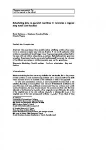
n this study the problem deals with number of jobs (𝑵 jobs ) to be processed on a number of identical parallel machines (𝒎 machines), when the objective is to minimize makespan (maximum completion time of the last job). The problem denoted by ( Pm | | C max ). Figure (1) shows (N) independent jobs on (𝑚) parallel machines.

limitations with a large number of jobs and when the number of machines are more than two.

IJSER

Fig. 1. (𝑚) parallel machines with (𝑁) jobs.

To solve the problem statement of this study, the following assumptions are used: 1. All machines are identical and are able to perform all operations. 2. Each machine can only process one task at a time. 3. Permission of a job on another machine is not allowed. 4. All jobs are available at time zero. There are many studies in literature dealing with parallel machines scheduling problems. Although the relatively small sized of identical parallel machines problems can be solved by operational methods such as dynamic programming, branch and bond method. However, these methods still have

2 LITERATUR REVIEW

Koulamas and Kyparisis proposed a modified longest processing time (MLPT) heuristic algorithm for the two uniform machine makespan minimization problem. The MLPT algorithm schedules the three longest jobs optimally first, followed by the remaining jobs sequenced according to the LPT rule. The obtained results showed that the MLPT rule has the tight worst-case bound of 1.22 [1], an improvement over the LPT bound of 1.28 [2]. Chaudhry et al presented a spreadsheet based on genetic algorithm approach to minimize the makespan for scheduling a set of tasks on identical parallel machines and worker assignment to the machines. The performance of the proposed approach is compared against two data sets of benchmark problems available on the internet. It was found that the proposed approach produces optimal solution for almost 95 percent of the problems demonstrating the effectiveness of the proposed approach [3]. Queiroz and Mendes addressed an identical parallel machines scheduling problem with release dates in which the total weighted tardiness has to be minimized. The obtained results showed that the instances of 10 jobs and 2 machines for which the metaheuristic achieved an optimal solution in a competitive amount of time, when compared with the exact approach. For the cases of 15 jobs and 3 machines and 20 jobs and 3 machines, the performance of the metaheuristic was similar [4]. A new method has been developed by Navid Hashemian to schedule jobs on parallel machines with availability constraints. The objective of the problem was to minimize the

IJSER © 2016 http://www.ijser.org


makespan of the total production schedule. It was concluded that the exact algorithm is able to solve large-scale problems which are not solvable by any other method including the current best ILP solver. Based on the results of the experiments for the ILP, it has been demonstrated that the proposed ILP can be used to solve the small-size problems effectively. The performance of the proposed algorithm is independent of the pattern of non-availability periods [5]. The aim of this study is to find the optimal schedule (solution) for identical parallel machines scheduling. This paper presented backtracking algorithm to find the optimal schedule (solution) for identical parallel machines scheduling. Also the paper suggested an algorithm to improve the initial solution.

3 PARALLEL MACHINES SCHEDULLING The aim of machine scheduling is to assign jobs to the machines based on related objective function to minimize operating time and increase productivity [6]. Parallel machines scheduling is the task of determining when each operation has to start and finish on each machine and using available resources in efficient manners to execute (assign) jobs or tasks on machines. The parallel machines can be identical (uniform) or unrelated. In this paper the case of study is identical parallel machines. Identical parallel machines are a set of machines which have the same speed factor and they can process all the jobs. Figure (2) shows Gantt chart for set of machines and jobs. Machines

M1

J1

M2

J3

J2

M3

J5

J6

J7

M4

J8

J9

J10

(3)

i=1,….,m , j=1,….,N

(4)

(5) The first equation (1) in the model is the objective function (C max ) makespan, which should be minimized. C max ≥ 0

Constraint (2) assures that the load on any machine is equal or less than ( Cmax ). Constraint (3) shows that each job must be assigned to exactly one machine. Constraint (4) describes the type of the assignment decision variable (

xij

=

xij ):

the job 𝑗 is assigned to machine 𝑖 { 01 ifif the job 𝑗 is not assigned to machine 𝑖

Constraint (5) shows that, the objective function

4 Solution method In this paper, the solution can be obtained in two steps: The LPT algorithm is used to find (generate) the initial solution, while the developed algorithm is used to improve the initial solution.

4-1 LPT algorithm The (LPT) algorithm always puts the smaller jobs towards the end of schedule, that makes it easier to balance the machines loads. According to the (LPT) algorithm, whenever one of the (m) machines is freed, the longest job among number of jobs (N) in decreasing order waiting for processing is selected to be next [16]. ∗

{ Li + p j : i = 1 , ..... , m }

(6)

pj

the processing

time of job ( j ). The makespan ( C max ) of any feasible solution is:

C max = max {Ci : i = 1 , ..... , m}

(7)

The steps of LPT algorithm are as follows: Step1: sort (N) jobs according to the non-increasing order of their processing time. Step 2: set ( j=1 ). Step 3: assign job ( j ) to machine (i) according to equation (6). Step 4: if j=N (all jobs are allocated) then go to the next step, otherwise set j=j+1 and go to the step 3.

: the assignment (decision) variable.

The mathematical model of the problem as follows:

Min C max subject to

Cmax is

integer variable.

Where: Li is the load on machine ( i ) ,

Time unit

𝑁 : number of jobs (integer). 𝑚 : number of machines. (integer). 𝑝𝑗 :processing time of job ( j ) (integer).

j =1

xij ∈ {0,1}

i ∗ = argmin

C max : the makespan (maximum completion time).

∑ p j xij ≤ C max

j=1,….,N

i =1

The next job (j) will be scheduled on machine ( i ) according to the equation:

J4

Assume that:

N

m

∑ xij = 1

IJSER

Fig. 2. Gantt chart for set of machines and jobs.

xij

354

(1)

LPT Step 5: calculate C max by using equation (7).

4-2 Developing the algorithm i=1,….,m

(2)

The developed algorithm, is used as a main algorithm and is based on two types of operations: (construction and



backtracking). The load of machines are determined in sequence, one after another. Therefore, the potential load of machine (i) with (1< i ≤ m) depends on the loads of the previous machines, then the loads on machines continue until assigning the last job [4]. Assume that, ( C max ): is the makespan of the current feasible solution. So if the optimal solution has not been explored yet, then its value is not greater than ( C max − 1 ) in the case of integer processing times. Therefore: (8)

UB = C max − 1

Where ( UB ) is the upper bound for the load of all machines in the feasible solution and still to be investigated. And the lower bound ( LB ) for all the other loads in the same feasible solution can be found by the following equation:  LB = max 0 , 

N

∑ pj j =1

 − (m − 1) UB  

(9)

Equation (9) implies that if all machines except one have a total load equal to the upper bound, then the remaining load is the lower bound. After finding a new feasible solution, both bounds (upper and lower bound) tighten up. To ensure that the load on any machine is feasible, the total load on the machine, must be between the lower and upper bounds. LB ≤

n

∑ p j k j ≤ UB j =1

355

The algorithm is always looking for the optimal solution. Therefore the backtracking is applied whenever any of the following two situations are accounted: 1- When the load of a machine is not feasible (cannot satisfy equation(10)). 2- When a new feasible solution has been found for all machines (updating makespan). When the machines has no further feasible load ( the load of machines are not satisfy equation (10) ). Then there is no feasible solution for the current upper bound and optimal makespan ( C

C

*

max

*

max )

is equal to pervious upper bound.

= UB + 1

(13)

4-3 Steps of the improvement algorithm: Step 1: set ( i = 1 ) and ( t = 1 ). Step 2: use (LPT) algorithm to find the initial solution (upper bound). Step 3: load machine (i) according to the equations (11) and (12). Step 4: if machine (i) does not satisfy inequality (10) go to step (6).

IJSER (10)

Where: ( k j ) is integer, and j =1,…..,n.

4-2-1 Construction phase There are many feasible solutions that can satisfy the equation (10). For an implicit enumeration procedure, the feasible solutions must be ordered somehow and enumerated in this order. One easy way to perform this task is to order them in lexicographical order also known as (the dictionary order) or (the alphabetic order). In the construction phase, and to load the machines one by one, the largest solution in the lexicographical order for (n) jobs types is given by equations (11) and (12). That is when the machine has no previous load.    UB   k1 = min   , r1  p    1   j −1     UB − ∑ p h k h    h =1  , r  , j = 2 ,....., n. k j = min    j pj        

(11)

Step 5: if (i =m) set ( UB = C max − 1 ) and ( t

step (3). otherwise set ( i

= t + 1)

and go to

= i + 1 ) and go to step (3).

∗ Step 6: calculate C max by using equation (13).

Step 7: print results and stop. Figure (3) shows the flow chart of the suggested algorithm.

5 Computer program The developed algorithms have been coded in MATLAB and executed on Intel (R) core (TM)i5 CPU 2.30 GHz, RAM 4.00 GH. System type (64bit) in order to remain comparable in terms of the computational time. The program is designed to solve variety of problems depending on number of machines (m) and number of jobs (N). Many computational applications with different levels of difficulties have been carried out to evaluate the performance of the suggested algorithm. 5-1 Case (1) Find the optimal schedule (solution) by using the (LPT) and the algorithms to minimize maximum completion time ( Cmax ) for (7) jobs their processing times ( p j ) given

(12)

The feasibility of the load is checked by equation (3-10). If the construction is successful (all machines are loaded and all conditions are satisfied), both the upper bound and lower bound are updated.

bellow: p j = [3, 3, 3, 4, 4, 5, 5 ]

4-2-2 Backtracking phase



356

Fig. (3). The flow chart of the algorithm. The jobs processed by (3) identical parallel machines, each machine can only process one job at any time and permission of a job on another machine is not allowed.

5-1-1 Using LPT algorithm to find the initial schedule (solution): Step1: sort the jobs in non-increasing order (5, 5, 4, 4, 3, 3, 3) Step 2: set j =1 Step 3: assign job (1) to the machine ( i ) according to equation (6).

start

Input No; of jobs (N) and their processing time. Input No; of machines ( )

i = argmin

{ Li + p j : i = 1 , ..... , m }

The load on machines: C1 = P1 + P5 + P7 = 5 + 3 + 3 = 11

i= 1 & t=1

C2 = P2 + P6 = 5+ 3 = 8

Use LPT algorithm to find initial solution UB =

C3 = P3 + P4 = 4+ 4 = 8 Step 4: j = N = 7 ( all jobs are assigned (allocated)).

IJSER Step 5: calculate

Cmax

by using equation (7).

Cmax = max {Ci : i = 1 , 2 , 3} → Cmax = max {C1 , C2 , C3 }

Load machine (i) according to formula (3-11) – (3-12)

Cmax = max {11 , 8 , 8}

→

C max = 11

The machines are loaded and the initial solution obtained by LPT algorithm are illustrated in Figure (4) by Gantt chart.

5-1-2 Using the algorithm to improve the initial solution: Step 1: set ( i = 1 ) and ( t = 1 ).

No

Machine (i) satisfy

Step 2: use (LPT) algorithm to find the initial solution (upper bound).

Yes

The lower bound ( LB ) can be found by equation (9) as follows:

No i=i+1

UB = Cmax = 11

At first iteration

i=m Yes

 LB = max 0 , 

∑ pj

 LB = max 0 , 

∑ pj

N

j =1

7

j =1

 − (m − 1) UB  

 − (3 − 1) 11 

→

LB = max {0 , 27 − (2) 11}

→

LB = max {0 , 5} → LB = 5

Step3: load machine(1) according to the equations (11) &(12).

UB = UB -1 and find (LB) by using equation (3-9)

   UB   k1 = min   , r1  p    1  

t=t+1 Calculate

by

using equation (3-13) & print results

stop

j −1     UB − ∑ p h k h    h =1  , r  , j = 2 ,....., n. k j = min   j   pj        

Therefore:


International Journal of Scientific & Engineering Research, Volume 7, Issue 3, March-2016 ISSN 2229-5518  11   k1 = min   , 2  5   

k2

→ k1 = min {2.2 , 2} →

2−1   UB − ∑ p h k h  h =1 = min  p2   

k1 = 2

    ,r  2 , j = 2      

→

   11 − ( p1 k1 )   k 2 = min   , 2 , j = 2 4       11 − (5 × 2)   k 2 = min   , 2 4    3−1   UB − ∑ p h k h  h =1 k 3 = min  p3   

→

→ k2 = 0

→ k3 = 0 Thus the load on

This means: the new upper bound is UB = 10 and the next iteration is t = 2 And the new lower bound ( LB )can be found by equation (9): With the same above procedure the new load on machines are: C1 = 10

Cmax

by using equation (3-7).

UB = C max − 1 → UB = 10 − 1 → UB = 9

and

t = t +1

→

t =3

This means: the new upper bound is UB = 9 and the next iteration is t = 3 And the new lower bound ( LB ) can be found by equation (9):

IJSER the new load on machines are: C1 = 9

j =1

3

C2 = 9

j =1

C3 = 9

then the machine(1) satisfy inequality (10) i = i + 1 → i = 1 + 1 → i = 2 ≠ m . then the next step is (3).

i =3 , m=3 → i =m

Step 3: load machine (2) according to the equations (11)&(12). With the same procedure for loading machine (1). The load on machine (2) is( C 2 ) as follows: M2 : C 2 = p1 k1 + p 2 k 2 + p3 k 3 → C 2 = 5 × 0 + 4 × 2 + 3 ×1 → C 2 = 11

Calculate C max by using equation (7).

C max = max {C1 , C 2 , C3 }

C max = max {9 , 9 , 9} → C max = 9

= t + 1 ).

3

Where the load on machine (2) is: C 2 = ∑ p j k j = 11

( UB = C max − 1 ) and ( t

j =1

UB = C max − 1

then the machine 2 satisfy inequality (10). i = i +1 → i = 2 +1 → i =3

UB = 9 − 1 → UB = 8 and

The load on machine(3) is ( C 3 ): M3 : C 3 = p1 k1 + p 2 k 2 + p3 k 3 → C 3 = 5 × 0 + 4 × 0 + 3 × 2 → C 3 = 6 Step 4: n

n

j =1

j =1

Where the load on machine (3) is: C 3 =

Cmax = max {Ci : i = 1 , ..... , m}

Cmax

t=4

This means: the new upper bound is UB = 8 and the next iteration is t = 4 Then the new lower bound ( LB ) can be found by equation (9): LB =11

C1 = 8 ; C2 = 8 , C3 = 8 Where the load on machines does not satisfy inequality (10). Then go to step (6)

3

∑ p j k j =6 j =1

∗

Step 6: set C max = UB + 1

Then the machine (3) satisfy inequality (10). Step 5: i = m = 3 then Calculate

t = t +1 →

the new load on machines are:

∑ p j k j ≤ UB ……. (3-10) → 5 ≤ ∑ p j k j ≤ 11

C max = max {Ci : i = 1 , 2 , 3}

→

LB = 9

n

Where the load on machine(1) is: C 1 = ∑ p j k j = 10

LB ≤

t = t +1

C max = max {10 , 8 , 9} → C max = 10

∑ p j k j ≤ UB ……. (3-10) → 5 ≤ ∑ p j k j ≤ 11 j =1

and

t=2

Calculate

M1 : C 1 = p1 k1 + p 2 k 2 + p3 k 3 → C 1 = 5 × 2 + 4 × 0 + 3 × 0 → C 1 = 10 n

UB = C max − 1 → UB = 11 − 1 → UB = 10

C3 = 9

machine(1) is ( C 1 ):

LB ≤

= t + 1 ).

C2 = 8

    ,r  3 , j = 3 →      

 11 − (5 × 2 + 4 × 0)   k 3 = min   , 3 , j = 3 3   

Step 4:

( UB = C max − 1 ) and ( t

LB = 7

k 2 = min { 0.25 , 2}

k 3 = min {0.33 , 3} , j = 3

357

by using equation (7).

C ∗max = 8 + 1 → C ∗max = 9 ∗ The optimal solution C max = 9 .

(7)

C max = max {C1 , C 2 , C3 } → C max = max {10 , 11 , 6} → C max = 11

Figure (4) shows Gantt chart for the solution and the load on machines .



358

The solution for case(1) by (LINGO, LPT and the suggested algorithm) LINGO Machine

Jobs

M1 P5 , P6 , P7 M2 P2 , P4 M3 P1 , P4 LPT algorithm Machine Jobs

Fig. (4). The optimal solution (schedule) for Case (1). Improving the initial solution to obtain the optimal solution (schedule) of the problem shown in figure (5).

C

C ∗max

Iteration

9 9 9

9

21

C

C ∗max

Iteration

M1 P1 , P5 , P7 M2 P2 , P6 M3 P3 , P4 the suggested algorithm Machine Jobs

11 8 8

11

1

C

C ∗max

Iteration

M1 M2 M3

9 9 9

9

4

P5 , P6 , P7 P2 , P4 P1 , P4

IJSER

And as can be observed the solution by LINGO and the

∗

algorithm program is identical ( C max = 9 ) with different distribution of jobs on machines and number of solution iterations.

4-4 Problems with random number of machines and jobs Number of problems with random number of machines and jobs have been generated to ensure and demonstrate effectiveness of the algorithm. Table (4-3) represents the results. TABLE 2 The solution for number of (m) Machines and (N) Jobs No 1 2 3 4

Mach -ines (m) 2 3 4 5

Jobs (N) 8 11 9 10

Iteration

C ∗max LINGO 42 26 12 25

LPT 42 28 15 25

Alg. 42 26 12 25

LINGO 17 72 88 260

Alg. 2 5 5 2

* Alg.: the suggested algorithm

Table (2) represents the results for random number of

Fig. (5). Using the suggested algorithm to Improve the initial solution. According to the results in table (4-1) the solution of the

∗

problem ( C max ) which obtained by LPT algorithm

(C ∗max = 11 ).

∗

machines and jobs, the makespan ( C max ) which obtained by LINGO and the algorithm for problem 1 and 2 in the table are equal. On the other hand there is a big difference, in the iterations to reach the solution, the algorithm is always faster than LINGO.

6 Conclusion: TABLE 1 IJSER © 2016 http://www.ijser.org

International Journal of Scientific & Engineering Research, Volume 7, Issue 3, March-2016 359 ISSN 2229-5518 In this study the ILP model introduced to represent and [9] C. H. Lin and C. Liao “Minimizing Makespan on Parallel Machines with Machine Eligibility Restrictions”, paper, The Open Operational formulate the problem( m max ), U-1 algorithm designed Research Journal, 2, pp. 18-24, 2008. [10] S. Kaya, “Parallel Machine Scheduling Subject to Machine and coded in MATLAB to solve the ILP model, also LINGO Availability Constraints”, MSc Thesis, Bilkent Uni., 2006. software has been used to test and evaluate performance of [11] G. ND. Jatinder , J. HO, and A. Ruiz-Torres "Makespan Minimization the suggested algorithm. on Identical Parallel Machines Subject to Mminimum Total FlowMany experiments and problems are used with random Time." Journal of the Chinese Institute of Industrial Engineers Vol. 21. No.3, pp. 220-229, 2004. number of machines (m) and jobs (N) to demonstrate [12] M. L. Pinedo, “Scheduling (Theory, Algorithms and Systems)”, New effectiveness of the algorithm solution. York University- USA, Fourth Edition, 2011. In this study, the ILP model can optimally be solved by ILP [13] K. Jihene and Y. Harrath “A Survey of Parallel Machine Scheduling solvers for small size of problems. And as can be observed Under Availability Constraints”, paper, International Journal of from tables (1) and (2) , LINGO can solve the problems with Computer and Information Technology, Vol. 3, issue 02, 2014. small size of number of machines and jobs. While the [14] I. Chaudhry, S. Mahmood and R. Ahmad ''Minimizing Makespan for Machine Scheduling and Worker Assignment Problem in Identical suggested algorithm can solve large sizes of parallel machines Parallel Machine Models Using GA'', Proc. of the World Congress scheduling problem optimally in small number of iteration. on Engineering, WCE 2010, June 30 - July 2, 2010, London, U.K. The results of the study demonstrated that: [15] M. L. Pinedo, “Planning and scheduling in manufacturing and 1- Efficiency and performance of the algorithm is evaluated services”, New York University- USA, 2005.

P | |C

by the number of iterations required to find the optimal solution. This good performance can be observed by varying the number of machines. 2- The number of feasible solution(s) which are generated is equal to number of iteration required to find optimal solution minus one (t-1) and each one of them is better than the previous one. 3- If the number of iteration (t=1) the initial solution obtained by LPT algorithm is optimal. It was found that computations required by LPT will escalate considerably as the number of machines increases. However, its capability is limited in terms of solving a large-scale problem.

REFERENCES [1 ]

[2]

[3]

[4]

[5]

[6]

[7]

[8]

IJSER

C. Koulamas and G. J. Kyparisis ''A modified LPT Algorithm for the Two Uniform Parallel Machine," European Journal of Operational Research, vol.196, pp.61–68, 2009. T. Gonzalez, T, O.H , Ibarra and S. Sahni '' Bounds for LPT Schedules on Uniform Processors'', SIAM Journal on Computing vol. 6, pp. 155– 166. I. Chaudhry, S. Mahmood and R. Ahmad ''Minimizing Makespan for Machine Scheduling and Worker Assignment Problem in Identical Parallel Machine Models Using GA'', Proc. of the World Congress on Engineering, WCE 2010, June 30 - July 2, 2010, London, U.K M. Queiroz and A. Mendes'' Strategies for Scheduling Jobs in an Identical Parallel Machine Production Environment, African Journal of Business Management, Vol. 7(16), pp. 1553-1559, 28 April, 2013. N. Hashemian'' Makespan ''Minimization for Parallel Machines Scheduling with Availability Constraints'', MSc dissertation, Dept. Industrial Engineering, Dalhousie Uni.,2010. B. V Reghavendra and A. N. Murthy “Workload Balancing in Identical Parallel Machines Scheduling Using Genetic Algorithm”, paper, ARPN Journal of Engineering and Applied Sciences. Vol.6, No.1, 2011. N. Hashemian'' Makespan ''Minimization for Parallel Machines Scheduling with Availability Constraints'', MSc dissertation, Dept. Industrial Engineering, Dalhousie Uni., 2010. C. Koulamas and G. J. Kyparisis ''A modified LPT Algorithm for the Two Uniform Parallel Machine," European Journal of Operational Research, vol.196, pp.61–68, 2009.
