Scripting Language for Java Source Code Recognition - ScienceDirect

Available online at www.sciencedirect.com

ScienceDirect IERI Procedia 10 (2014) 119 – 130

20014 Internattional Confe ference on Future F Inform mation Enggineering

Scrippting Lannguage for f Java Source Code C Reecognitioon Tomáš Bublík*, B M Miroslav Viirius Faaculty of Nuclear Sciences and Phyysical Engineerinng Czech Techniccal University in Prague, P Trojanovva 13, Prague, 1220 00, Czech Republic

Absttract This paper presentss general results on the Java source s code sniippet detection problem. We propose p the toool which uses m detection. A number of sollutions for all of these tasks have been prooposed in the graphh and subgraphh isomorphism literaature. Howeverr, although thaat all these soluutions are reallly fast, they co ompare just thhe constant stattic trees. Our soluttion offers to ennter an input saample dynamiccally with the Scripthon S langu uage while presserving an acceeptable speed. We used u several opttimizations to achieve a very low w number of coomparisons duriing the matchinng algorithm. © 2014 The Authors. Published by Elsevier B.V. This is an open access article under the CC BY-NC-ND license © 20014. Publishedd by Elsevier B.V. (http://creativecommons.org/licenses/by-nc-nd/3.0/). Sele ection and peer review undeer responsibilitty of Informattion Engineering Research Institute Selection and peer review under responsibility of Information Engineering Research Institute Keyw words: AST; Java; tree matching; Scriphon; S source code recognition

1. Introduction I Itt is usual thaat programs, consisting off a large souurce code, aree becoming chaotic, c and many times desccribed illnessees start to apppear (code duuplicity, weakk reusability, etc.). Maintaaining a sourcce code is a serioous issue. Theere are a lot of o tools and guides g on how w to approach h this issue. The T tool, descrribed in this workk, serves to prrogrammable Java source code c scanning. This tool is based b on the Scripthon S langguage which was developed for these purposses in the scoppe of this worrk. A script, which w describees a source coode structure and its propertiess, can be wriitten in this laanguage. This allows defiining dynamicc properties oof searching

* Corresponding author. a Tel.: +4200605155484. E E-mail address: toomas.bublik@gm mail.com.

2212-6678 © 2014 The Authors. Published by Elsevier B.V. This is an open access article under the CC BY-NC-ND license (http://creativecommons.org/licenses/by-nc-nd/3.0/). Selection and peer review under responsibility of Information Engineering Research Institute doi:10.1016/j.ieri.2014.09.100

120

Tomáš Bublík and Miroslav Virius / IERI Procedia 10 (2014) 119 – 130

requirements. Next, an abstract syntax tree (hereinafter AST) is created dynamically from this script. Meanwhile, a similar tree is created from given Java source, and these two trees are matched by a graph matching algorithm. However, not only graph shapes are compared, also trees properties are considered. To obtain results faster, several graph optimizations are used during this process. And it is possible to scan higher amount of source code classes during a relatively short time. Typical usage of this approach is as follows: A user wants to find something, not easily describable, in a large program. But he or she knows that it could be there. He or she can use our tool and try to find at least the similar snippet of indented code. Therefore, a user performs a searching procedure, and specifies the input script based on the received results. By repeating this procedure, he or she filters the unintended results, and finally gets the desired code snippet. Our tool is useful not just for the fast Java sources scanning, but for example, for a better definability of search conditions. Another usage area of our tool can be a clone’s detection problem. By using other clones detection tools, a material for further research can be gathered. For example, the non-ideal clones are difficult to detect and the output of such programs isn’t unequivocal in many cases. However, it can be classified by Sripthon, and a common searching script based on such output can be. 2. Theory A graph is an ordered pair ࡳ ൌ ሺࢂǡ ࡱሻ where ࢂ is a finite, non-empty set of objects called vertices, and ࡱ is a (possibly empty) set of unordered pairs of distinct vertices i.e., 2-subsets of ࢂ called edges. The set ࢂ is called the vertex set of ࡳ, and ࡱ is called the edge set of ࡳǤ If ࢋ ൌ ሼ࢛ǡ ࢜ሽ ‫ࡱ א‬ሺࡳሻ, we say that vertices ࢛ and ࢜ are adjacent in ࡳ, and that ࢋ࢐࢕࢏࢔࢙࢛ and ࢜. We’ll also say that ࢛ and ࢜ are the ࢋ࢔ࢊ࢙ of ࢋ. The edge ࢋ is said to be ࢏࢔ࢉ࢏ࢊࢋ࢔࢚ with ࢛ (and ࢜), and vice versa. We write ࢛࢜ (or ࢛࢜) to denote the edge ሼ࢛ǡ ࢜ሽ, on the understanding that no order is implied. Two graphs are ࢋ࢛ࢗࢇ࢒ if they have the same vertex set and the same edge set. But there are other ways in which two graphs could be regarded the same. For example, one could regard two graph as being “the same” if it is possible to rename the vertices of one and obtain the other. Such graphs are identical in every respect except for the names of the vertices. In this case, we call the graphs ࢏࢙࢕࢓࢕࢘࢖ࢎ࢏ࢉ. Formally, graphs ࡳ and ࡴ are isomorphic if there is a ૚ െ ૚ correspondence ࢌǣ ࢂሺࡳሻ ՜ ࢂሺࡴሻ such that ࢞࢟ ‫ࡱ א‬ሺࡳሻ ՞ ࢌሺ࢞ሻࢌሺ࢟ሻ ‫ࡱ א‬ሺࡴሻ. This function ࢌ is called an isomorphism. A tree is a connected graph that has no cycles (i.e., a connected acyclic graph). The graph matching problem is actually the same as the problem of finding the isomorphism between the graphs. Moreover, matching the parts of a graph with a pattern is the same challenge as the finding the isomorphic subgraph. There are many approaches to this topic in Irniger et al., 2005. Subgraph isomorphism is useful to find out if a given object is part of another object or even of a collection of several objects. The maximum common subgraph of two graphs ࢍ૚ and ࢍ૛ is the largest graph that is isomorphic to a subgraph of both ࢍ૚ and ࢍ૛ . Maximum common subgraph is useful to measure the similarity of two objects. Algorithms for graph isomorphism, subgraph isomorphism and maximum common subgraph detection have been reported in McKay, 1981, Ullmann, 1976, Levi, 1972, McGregor, 1982.. A more general method to measure the similarity of two graphs is graph edit distance. It is a generalization of string edit distance, also known as Levenshtein distance Stephen 1994. Another approach measuring the similarity of two graphs is a distance measure based on the maximum common subgraph between ࢍ૚ and ࢍ૛ . With increasing work being done in the field of maximum common subgraph detection, these measures are growing in popularity. In Bunke et al., 1998, a graph distance measure based on the maximum common subgraph of two graphs is introduced. It is shown that the well-known concept of maximum common subgraph distance is a special case of graph edit distance under particular edit costs. Consequently, algorithms originally developed for maximum common subgraph detection can be used for edit distance computation and vice versa for the considered edit

Tomas Bublik and Miroslav Virius / IERI Procedia 10 (2014) 119 – 130

costs. Furthermore, in Fernandez et al., 2001 the concepts of maximum common subgraph and minimum common supergraph are combined to derive a graph distance measure and in Wallis et al., 2001, graph distances based on the minimum common supergraph denoted as the ࢍ࢘ࢇ࢖ࢎ࢛࢔࢏࢕࢔ are discussed. A number of graph matching algorithms are known from the literature Sanfeliu et al., 1983, Tsai et al., 1979, Eshera et al., 1984, Wong, 1990. All of these methods are guaranteed to find the optimal solution, but require exponential time and space. Suboptimal or approximate methods, on the other hand, are polynomially bound in the number of computation steps, but may fail to find the optimal solution. In Wilson et al., 2004, inexact graph matching is performed by calculating the Levenshtein distance on the eigenvectors of the graphs. Another approach illustrated in Robles et al., 2005 converts the adjacency matrix into a string, then uses the leading eigenvector to impose a serial ordering on the string. Graphs are then matched by applying string matching techniques to their string representation. A different idea is pursued in Caelli et al., 2004, Caelli et al., 2004 where eigen(sub)space projections and vertex clustering methods are explored. Whereas in Caelli et al., 2004 the objective of the method is to work in the eigenspace of the graphs, in Caelli et al., 2004 subgraphs are matched based on their vertex connectivities defined in the common subspace. 3. Other Solutions There exists a lot of searching types which can be used to detect a clone Roy et al., 2009. The textual approaches belong to basic ones. These approaches are easy to implement, on the other hand, because of a large excess of non-program material contained in source code, they suffer from a whole range of ailments. For example, checking a variable scope could be very challenging issue by using textual comparisons. The token-based comparisons are the next group of approaches needs to be considered. This kind of approaches divides a source code into the tokens sequences which are compared to each other. This is little more robust than the textual ones, because it doesn’t work with unnecessary text material like spaces, comments etc. However, this approach still does not handle a variable or a method scope. More effective algorithms are the tree-based. There exist two approaches to them: metric-based and treebased. The metric-based ones use the Java source generated metrics. These metrics are then compared with the metric generated from original sources. The tree-based methods are base on abstract syntax subtrees comparison. These methods are used in our work. They are little more difficult to implement, but they are very effective and they offers more searching options. On contrary, the algorithms based on these methods are more time consuming comparing to other types. Ira D. Baxter was a pioneer in this area Baxter et al., 1998. He proposed a solution using the subtrees hashing into the buckets. And only the same bucket trees are being compared. Another solution proposed Wahler et al., 2004. He converted AST into XML and applied data mining techniques on it. The remaining question is the speed of XML processing procedures. Further, an interesting option proposed Koschke et al., 2006. They serialized generated AST and compared just the suffix tree tokens of it. The proposed algorithm is very fast. It is able to detect a clone in a linear time. The lack of these algorithms is the inability to detect snippets dynamically. They suppose a constant and unchanging original pattern. On the opposite, our solution offers the usage of the dynamic input based on a scripting language. This means that the input could be conditioned or iterated, and the searching tree changes according to the searched tree properties. Even the variables can be used. For example, a user can declare the “clazz” variable of type Class, and use it later for the name comparison: Class clazz Block(StmtNum=2)

121

122

Tomáš Bublík and Miroslav Virius / IERI Procedia 10 (2014) 119 – 130

if (clazz.Name=="HelloWorld") ... else ...

This example means that we search the class with two statements inside, and if the name of this class is “HelloWorld”, then we search something, else we search something else. 4. Scripthon language Within this work, a new programming language named Scripthon, capable of these functionalities, was developed. Using this language, it is possible to describe a code structure with properties, and it is even possible to change the properties of a searching sample in dependence of searched segment properties. Scripthon is a dynamically typed, interpreted, and non-procedural language. Its translation into a treeexpressing form and its usage is very similar to the usage of any other modern script languages. The complete definition of the Scripthon language semantics is beyond the scope of this paper, can be found in Bublík et al. 2012. Because the language is designed to be just a scripting language, there are no special constructions starting a script. This language is neither a pure object-oriented language. The input for a compiler is a text with a sequence of commands. This sequence describes consecutive statements in Java source code. Commands with a variable detail degree correspond to a variable length code segment. A detail level is not fixed, and can vary in every command. One command can correspond to a line of source code; other one can describe a whole class in Java. A Scripthon structure is very similar to the structures of the others contemporary dynamic programming languages. Individual commands are separated by lines. There is no command separator in Scripthon. Inner parts of blocks are tab nested. A block is not delimited by any signs; just a hierarchy of tabulators is used. Looking for a method with a specific name? Suppose we have the most common Java code: public class HelloWorld { public static void main(String[] args) { System.out.println(args); } } Let’s suppose we are looking for the method named “main”. It’s easy. A user just starts a text search dialog (usually by CTLF + F shortcut) and performs a searching procedure. Unfortunately, this will find a lot of miscellaneous results. With Scripthon, we can search just methods: Meth(Name=”main”) Moreover, we want just the public and static ones: Meth(Name=”main”; Rest=[public, static]) Even more, the most specific searching criteria for the main method are: Meth(Name="main"; Rest=[public, static]; Ret=void; ParNum=1; ParNames=["args"]) With Scripthon, we can define a method call inside the main method:

ParTypes=[String[]];

Tomas Bublik and Miroslav Virius / IERI Procedia 10 (2014) 119 – 130

Meth(Name=”main”; Rest=[public, static]) MethCall(Name="System.out.println";Params=["args"]) Scripthon supports also a block of code description. We can define properties of block by this way: Class(Name="HelloWorld") Meth(Name=”main”) Block(StmtNum=1;Order=false) Again, this example corresponds to a given “hello world” example. There is one statement inside the main method and the order of statements doesn’t matter. Another interesting Scripthon’s keyword is the word “Any”. It is useful for an indefinite searching. It means the searched statements can be anything, or empty. To describe the code above, we can write:  Meth(Name=”main”) Any() But the desired code can look like this:  public static void main(String[] args) { int i = 1; i++; System.out.println(args); } And we can find this by the following script: Meth(Name=”main”) Any() MethCall(Name="System.out.println") There are several more keywords supported by Scripthon. For example, Init() for a variable initialization, Loop() for a common loop, etc. Finally, with the presented examples, it is easy to find a singleton in code: Class() class Block(Order=false;Consecutive=false) Meth(Name=class.Name;Rest=private) MethCall(Ret=class.Name;Rest=[public, static]) The only unmentioned parameter here is the “consecutive” parameter. It means that the statements inside block must not be consecutive. These statements just need to be contained somewhere in the given block. 5. Obtaining optimized trees The Java Compiler API is used to get AST from the given Java sources in the first iteration. This API is free and is contained in Java SDK. It provides access to control the Java compiler, and one of the compilation outputs is an abstract syntax tree of the given sources. Just one condition needs to be met. The Java sources must be compilable. While browsing the Java source code, the tree, with the nodes enhanced by four numbers, is created. These numbers are the natural numbers named left, right, level and level under. The first and the second number (left, right) denote the order index of a node in the tree preorder traversal. Therefore, an ancestor’s left index is always smaller than its children left index, while the right index is always bigger than any children’s right index. The level number denotes the level in a tree hierarchy of vertices, and the level under number denotes a

123

124

Tomáš Bublík and Miroslav Virius / IERI Procedia 10 (2014) 119 – 130

number of levels under the current node (compare with the method described in Yao et al., 2004). Suppose that ‫ ݔ‬and ‫ ݕ‬are two nodes from a tree; the following rules are valid for these values. x The node is an ancestor of šand šis a descendant of if ›Ǥ Ž‡ˆ– ൏ ‫ݔ‬Ǥ Ž‡ˆ– ൏ ‫ݕ‬Ǥ ‫ݐ݄݃݅ݎ‬ x The node is a parent of šand is a child of if 1) ›Ǥ Ž‡ˆ– ൏ ‫ݔ‬Ǥ Ž‡ˆ– ൏ ‫ݕ‬Ǥ ‫ ݐ݄݃݅ݎ‬and 2) ›Ǥ Ž‡˜‡Ž ൌ šǤ Ž‡˜‡Ž െ ͳ x The node has ሺሺšǤ Ž‡ˆ– െ šǤ ”‹‰Š–ሻ െ ͳሻ sub-nodes. All these data are acquired during a single pass through the tree. Obtaining this information is not a time consuming operation, because it is made during the tree production process. On the other hand, the number of comparisons can be significantly reduced with these numbers.

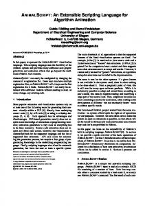
Fig. 1.

Example of AST with indexes

Fig. 2.

Node “main” with one child

With this information (Fig. 1), we know how many children are contained in the currently processing node, or whether a node is a leaf. Thanks to it, a lot comparisons need not to be performed. For example, comparing this script: Meth(Name=”main”) Block(StmtNum=4) with this Java code: public static void main(String[] args) {

Tomas Bublik and Miroslav Virius / IERI Procedia 10 (2014) 119 – 130

System.out.println(args); } means that these two nodes are compared (Fig. 2.) But the left and right indexes signalizes that the “main” node does have just one child, however, we search for a method with 4 statements. So that, this code does not corresponds to the script, and any other comparisons are not needed. 6. Comprehensive description of solution The complete process is little bit complex, but the top overview is easy. Before the main matching procedure,

Fig. 3.

Complete process

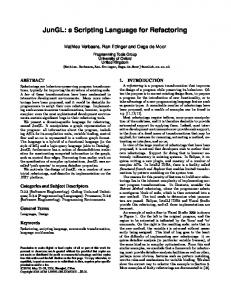
Fig. 4.

Indexing of nodes

two processes take place. The first one starts immediately after a user enters a Java sources path. It compiles and optimizes AST obtained from the sources. This process is done just once, because the sources are always the same in scope of this process. It runs on the background. The second process starts immediately after a user enters a searching script. It compiles the script and, if it is not done, waits for the first process. Next, the first iteration is performed. Matching is performed together with index building during this iteration. After that, results are presented to a user. It is supposed that a user improves the entered script according to the results. And then the algorithm runs again with only difference. Only the nodes corresponding to the index of changed Scripthon part are considered.

125

126

Tomáš Bublík and Miroslav Virius / IERI Procedia 10 (2014) 119 – 130

Figure 4 shows how the indexing works. Let’s suppose the same “HelloWorld” example from the beginning of this paper. The index into the group of corresponding Java sources is assigned to all non-leaf nodes. When a user changes the input script, the new and the old corresponding trees are compared. In our example (Fig. 4), the “System.out.println” method call was changed to the initiation the variable “i” of type int. This is indicated by gray colour. The node which contains this change is then detected by the tree matching algorithm. It is clear that the set of corresponding Java sources to this node remains the same. Therefore, only this set needs to be considered in the next search iteration. These top level listings shows how the matching algorithm works: 1 for(Class c from classes) 2 for (Statement s from statements) 3 match = compare(c.node, s) 4 if (!match) 5 break 6 if (match) 7 addToResults(c) 8 9 compare(Node n, Statement s) 10 match = optiMatch(n, s) 11 if (match) 12 if (n.allProperties matches s.allProperties) 13 addResultsForThisStatement(n, s);

14 for (n.children, s.children) 15 match = compare(...) 16 if (!match) 17 return false 18 else return false 19 return match 20 21 optiMatch(Node n, Statement s) 22 checkTreeSizes(n, s) 23 checkLevels(n, s) 24 checkChildrensNumber(n, s) 25 return resultOfChecks

All the source classes are iterated in a loop (line 1). Next, all the Scripthon statements are then iterated inside this loop (line 2). The “compare” method is called inside the second loop. This method compares all the sub-statements with the node from the outside loop. If there is a match, the founded result is added to the group of results (line 7), otherwise the inner loop is beaked (line 5). According to the line 15, the “compare” method calls itself recursively. First, it checks the match with prepared optimizations (line 10). The “optiMatch” method (line 21) checks the structure of trees and tries to exclude the node by tree sizes mismatch, by levels number mismatch or children number mismatch. If the “optiMatch” method return false, then the node is excluded from further considerations (line 18). On contrary, when the optimizations do not exclude the node, all the children of the statement and node are compared in the “compare” recursive call (line 15). But before that, we know about the correspondence between the current statement and the current node, therefore it is saved into memory on the line 13. If the entire children set matches, the current node is considered equal, and true is returned from the “compare” method (line 19). Otherwise, false is returned (line 17). Finally, if is the node equals to all the Sripthon statements, it is saved into the results set (line 7). 7. Complexity analysis Because the non-constant trees are compared, the complexity determination of our algorithm is not an easy task. Syntax trees are always little bit different and since we compare the characteristics of the nodes according to a user input, the comparison is always different. To begin, it is possible to emerge from the complexity of the subtrees comparing algorithm. The subtree comparison problem is NP-hard. And according to Valiente, 2002, the complexity isܱሺሺ݊ଵ ൅  ݊ଶ ሻଶ ሻ, where ݊ଵ is number of the first tree nodes whereas ݊ଶ is number of the second tree nodes. There exist also several improvements Shamir et al., 1999. Our algorithm, however, is based on the use of information on the required sample tree. Thanks to this information, a lot of comparisons can be saved. Moreover, the whole tree is traversed just once during the first

127

Tomas Bublik and Miroslav Virius / IERI Procedia 10 (2014) 119 – 130

run. During next runs, just the data, corresponding to the node containing the change, are considered. Unfortunately, also the commands increasing the comparisons number can be written in Scripthon. For example: Any() MethCall(Name="someName") This script must run over all statements in the source code up to the “someMethod” method. If the code before this method is large, several more comparisons must be done. And moreover, it must be done even in the case if there is no such method. This means ݊ more comparisons in the worst case. Another example: Block(Order=false) This command identifies the statements in a block. But if the statements order doesn’t matter, the algorithm must compare all the children of the “Block” node. If the first statement corresponds to the last child, there will be ݊ more comparisons. And if the second statement corresponds to the penultimate child, there will be ݊ െ ͳ more comparisons. In conclusion, there could be ̱݊ଶ more comparisons in the worst case. To assess whether the implemented optimization makes sense, the algorithm is equipped with the ability to switch off the optimization globally. If we note how many comparisons actually occur in the case of enabled optimizations, we obtain the basis to assess whether our optimization are meaningful. We chose a project with 800 Java classes as a test sample. Then several search iteration were run over this project. When testing with disabled optimizations, nodes 142 275 comparisons were performed. On the other hand, with enabled optimization, there was a big difference between the first run, with index gathering function, and the following rounds, with using this index. In the first case, there were 28 268 comparisons, whilst in the second case, there were 6 800. As can be seen, the second comparisons numbers are much lower. 8. Results A quite common computer with Windows 7, 2,4 GHz CPU and 8 GB memory was used to test the time complexity of our algorithm. Used Java version was 1.7.0_51. To show real benefits of our solution, we performed several search procedures with disabled and also with enabled optimizations. We tried to identify several important parts which could, by their time, reflect the actual contribution of the whole work. Without optimizations, the algorithm runs over all input classes by the “brute force” method. In this case, no results caching and no indexing was used. We compared the obtained times with times of optimized algorithm version in Table 1. Table 1 Times table First round Time of Java compilation Time of Scripthon compilation Time of search Total time Second round Time of Java compilation Time of Scripthon compilation

Without optimizations

Optimized

38 469 ms

39 542 ms

35 ms

33 ms

962 ms

170 ms

39 441 ms

39 924 ms

Without optimizations

Optimized

0 ms

0 ms

48 ms

44 ms

128

Tomáš Bublík and Miroslav Virius / IERI Procedia 10 (2014) 119 – 130

Time of search Time of search with change detection Total time Total time with change detection

888 ms

151 ms

68 ms

15 ms

1 062 ms

208 ms

118 ms

62 ms

As can be seen from the tables, measurements were carried out in two phases. The first table shows the times received always in the first run of the algorithm. Both tables have two columns to indicate whether the time was with or without the optimizations. The first significant difference is the time of compilation which is not used in the second run. It is zero, because it does not occur in further runs. Next row represents the times of Scripthon code compilation process. Because there weren’t significant differences between the searching scripts, these times are almost the same. Another row shows the times of the own matching process. There is a big difference between these times. Optimized version is about 5 times faster, however, according to the first table, this time is completely lost in the compilation time. To make matters worse, the total time is even bigger than the time without any optimization! The second table contains one more row. This row shows the time of matching process with help of the index created in previous runs. In this case we used this script: Class() Any() Meth(Name="add") Init(Name="errors") For the further runs, the only change was a name in the “Init” statement. The algorithm used just the nodes corresponding to “Meth(Name=”add”)” in this case. In other words, the algorithm considered just the classes with methods named “add”. As can be seen, if there is no need to compile the entire sources again, and if the algorithm has an index created from the previous runs, the matching time acceleration is enormous. Then the complete process runs for a tiny fraction of the time needed to run the same task without any improvement. 9. Conclusion Our project showed that the source recognition can be speeded up highly. The significant contribution for the speed is the caching the nodes corresponding to statements. Although this approach speeded up the process, however, it is necessary to say that this applies just for further runs. In the case of the first runs, compilation of sources takes a lot of time. But there exist a lot of improvements. For example, the compilation can start already during script wring. This project shows the usability of programmable and dynamic code recognition in an acceptable time. Currently, the project is used just for science purposes, but we want to add all the workaround to make it other users. We consider also the use of the tree indexing methods to achieve even a higher speed of the matching process in the future.

Acknowledgements This work is supported by the SGS11/167/OHK4/3T/14 grant of the Ministry of Education, Youth and Sports of the Czech Republic.

Tomas Bublik and Miroslav Virius / IERI Procedia 10 (2014) 119 – 130

References [1] Tomáš Bublík., Miroslav Virius. New language for searching Java code snippets. In: ITAT 2012. Proc. of the 12th national conference ITAT. diar, Sep 17 – 21 2012. Pavol Jozef Safrik University in Kosice. p. 35 – 40. [2] Christophe-André M. Irniger. Graph Matching - Filtering Databases of Graphs Using Machine Learning Techniques. 2005, ISBN 1-58603-557-6. [3] B.D. McKay. Practical graph isomorphism. In Congressus Numerantium, volume 30, 1981, pages 45–87. [4] J.R. Ullmann. An algorithm for subgraph isomorphism. Journal ofthe Association for Computing Machinery, 1976, pages 31-42. [5] G. Levi. A note on the derivation of maximal common subgraphs oftwo directed or undirected graphs. Calcolo, 1972, pages 341-354. [6] J. McGregor. Backtrack search algorithms and the maximal commonsubgraph problem. SoftwarePractice and Experience, 1982, pages 23-34. [7] G.A. Stephen. String Searching Algorithms. World Scientific, 1994. [8] H. Bunke and K. Shearer. A graph distance metric based on the maximalcommon subgraph. Pattern Recognition Letters, 1998, pages 255-259. [9] M.-L. Fernandez and G. Valiente. A graph distance metric combining maximum common subgraph and minimum common supergraph. Pattern Recognition Letters, 2001, pages 753-758. [10] W.D. Wallis, P. Shoubridge, M. Kraetz, and D. Ray. Graph distances using graph union. Pattern Recognition Letters, May 2001, pages 701-704. [11] A. Sanfeliu and K.S. Fu. A distance measure between attributed relationalgraphs for pattern recognition. IEEE Transactions on Systems, Man, and Cybernetics, 1983, 353-363. [12] W.H. Tsai and K.S. Fu. Error-correcting isomorphisms of attributedrelational graphs for pattern recognition. IEEE Transactions on Systems, Man, and Cybernetics, 1979, pages 757-768. [13] M.A. Eshera and K.S. Fu. A graph distance measure for image analysis. IEEE Transactions on Systems, Man, and Cybernetics, 1984, pages 398-408. [14] E.K. Wong. Three-dimensional object recognition by attributed graphs. In H. Bunke and A. Sanfeliu, editors, Syntactic and Structural Pattern Recognition- Theory and Applications, World Scientific, 1990, pages 381-414. [15] R. Wilson and E.R. Hancock. Levenshtein distance for graph spectral features. In J. Kittler, M. Petrou, and M. Nixon, editors, Proc. 17th Int. Conference on Pattern Recognition, volume 2, 2004, pages 489-492. [16] A. Robles-Kelly and E.R. Hancock. Graph edit distance from spectral seriation. IEEE Transactions on Pattern Analysis and Machine Intelligence, 2005, pages 365-378. [17] T. Caelli and S. Kosinov. Inexact graph matching using eigensubspace projection clustering. Int. Journal of Pattern Recognition and Artificial Intelligence, 2004, pages 329-355. [18] T. Caelli and S. Kosinov. An eigenspace projection clustering method for inexact graph matching. IEEE Transactions on Pattern Analysis and Machine Intelligence, 2004, pages 515-519. [19] Ch. K. Roy, J. R. Cordy, and R. Koschke. 2009. Comparison and evaluation of code clone detection techniques and tools: A qualitative approach. Sci. Comput. Program. 74, 7 (May 2009), pp. 470-495. [20] I. D. Baxter, A. Yahin, L. Moura, M. Sant'Anna, and L. Bier. 1998. Clone Detection Using Abstract Syntax Trees. In Proceedings of the International Conference on Software Maintenance (ICSM '98). IEEE Computer Society, Washington, DC, USA, pp. 368-377. [21] R. Koschke, R.Falke, P. Frenzel. Clone Detection Using Abstract Syntax Suffix Trees, Reverse Engineering. 2006. WCRE '06. 13th Working Conference on, ISBN 0-7695-2719-1, 2006, pages 253-262. [22] J. T. Yao and M. Zhang. 2004. A Fast Tree Pattern Matching Algorithm for XML Query. In Proceedings of the 2004 IEEE/WIC/ACM International Conference on Web Intelligence (WI ’04). IEEE Computer Society, Washington, DC, USA, pp. 235-241. [23] G. Valiente. Algorithms on Trees and Graphs. Springer, ISBN 3540435506, 2002, page 170.

129

130

Tomáš Bublík and Miroslav Virius / IERI Procedia 10 (2014) 119 – 130

[24] V. Wahler, D. Seipel, J. W. von Gudenberg, and G. Fischer. Clone detection in source code by frequent itemset techniques. In SCAM, 2004. [25] R. Shamir, D. Tsur. Faster Subtree Isomorphism. In Journal of Algorithms, Volume 33 Issue 2, 1999, pages 267-280, doi:10.1006/jagm.1999.1044