SDPT3 — A Matlab software package for semidefinite programming ...

Optimization Methods and Software

ISSN: 1055-6788 (Print) 1029-4937 (Online) Journal homepage: http://www.tandfonline.com/loi/goms20

SDPT3 — A Matlab software package for semidefinite programming, Version 1.3 K. C. Toh , M. J. Todd & R. H. Tütüncü To cite this article: K. C. Toh , M. J. Todd & R. H. Tütüncü (1999) SDPT3 — A Matlab software package for semidefinite programming, Version 1.3, Optimization Methods and Software, 11:1-4, 545-581, DOI: 10.1080/10556789908805762 To link to this article: http://dx.doi.org/10.1080/10556789908805762

Published online: 30 Jan 2008.

Submit your article to this journal

Article views: 518

View related articles

Citing articles: 619 View citing articles

Full Terms & Conditions of access and use can be found at http://www.tandfonline.com/action/journalInformation?journalCode=goms20 Download by: [NUS National University of Singapore]

Date: 16 June 2017, At: 20:40

Optirniration Meth. & Sofl., 1999, Vol. 11Br12, pp. 545-581 Reprints available directly from the publisher Photocopying permitted by license only

@ 1999 OPA (Overseas Publishers Association)

N.V.

Published by license under the Gordon and Breach Science Publishers imprint. Printed in Malaysia.

SDPT3 - A MATLAB SOFTWARE PACKAGE FOR SEMIDEFINITE PROGRAMMING, VERSION 1.3 K. C. TOHal*,M. J. T O D D ~and ~ ~R. H. TUTUNCU~.~ aDepartment of Mathematics, National University of Singapore, 10 Kent Ridge Crescent, Singapore 119260; b ~ c h o oof l Operations Research and Industrial Engineering, Cornell University, Ithaca, New York 14853, USA; 'Department of Mathematical Sciences, Carnegie Mellon University, Pittsburgh, PA 15213, USA (Received 3 February 1998; Revised 18 August 1998; In final form 25 August 1998) This software package is a MATLABimplementation of infeasible path-following algorithms for solving standard semidefinite programs (SDP). Mehrotra-type predictor-corrector variants are included. Analogous algorithms for the homogeneous formulation of the standard SDP are also implemented. Four types of search directions are available, namely, the AHO, HKM, NT, and GT directions. A few classes of SDP problems are included as well. Numerical results for these classes show that our algorithms are fairly efficient and robust on problems with dimensions of the order of a hundred.

1 INTRODUCTION

This is a software package for solving the standard SDP:

(P)

minxC

X

* Corresponding Author: E-mail: [email protected]. Research supported in part by National University of Singapore Academic Research Grant RP972685. t E-mail: [email protected]. Research supported in part by NSF through grant DMS-9505155 and ONR through grant N00014-96-1-0050. i E-mail: [email protected]. Research supported in part by NSF through grant DMS-9706950.

546

K. C. TOH et al.

where Ak E 'Hn, C E 'Hn and b E Rm are given data, and X E 'Hn is the variable, possibly complex. Here 'Hn denotes the space of n x n Hermitian matrices, P Q denotes the inner product Tr(P*Q), and X k 0 means that X is positive semidefinite. We assume that the set { A l , . . . , Ak) is linearly independent. (Linearly dependent constraints are allowed; these are detected and removed automatically. However, if this set is nearly dependent, transformation to a better-conditioned basis may be advisable for numerical stability.) The software also solves the dual problem associated with (P):

where y E Rm and Z E 'Fln are the variables. This package is written in MATLAB version 5.0. It is available from the internet sites: http : //www.math.nus.edu.sg/"mattohkc/index.html http : //www.math.cmu.edu/Yeha/sdpt3.html

The purpose of this software package is to provide researchers in SDP with a collection of reasonably efficient and robust algorithms that can solve general SDPs with matrices of dimensions of the order of a hundred. If your problem is large-scale, you should probably use an implementation that exploits problem structure. The only structure we exploit in this package is block-diagonal structure, where MATLABcell arrays are used to handle dense and sparse blocks separately. We hope that researchers in SDP may benefit from the algorithmic and computational framework provided by our software in developing their own algorithms. We also hope that the computational results provided here will be useful for benchmarking. To facilitate other authors in evaluating the performance of their own algorithms, we include a few classes of SDP problems in this software package as well. A special feature that distinguishes this SDP software from others (e.g., [4,6,9,24]) is that complex data are allowed, a feature shared by the SeDuMi code of Sturm [19]. But note that b and y must be real. Another special feature, though also shared by the software of [9], of our package

SDPT3-MATLABSOFTWARE PACKAGE

547

is that the sparsity of matrices Ak is exploited in the computation of the Schur complement matrix required at each iteration of our SDP algorithms. Part of the codes for real symmetric matrices is originally based on those by Alizadeh, Haeberly, and Overton, whose help we gratefully acknowledge.

2 INFEASIBLE-INTERIOR-POINT ALGORITHMS 2.1 The Search Direction For later discussion, let us first introduce the operator A defined by

The adjoint of A with respect to the standard inner products in 'Hn and Rm is the operator

The main step at each iteration of our algorithms is the computation of the search direction (AX, Ay, AZ) from the symmetrized Newton equation (with respect to an invertible matrix P which is usually chosen as a function of the current iterate X , Z) given below.

where p = X 0 Z/n and a is the centering parameter. Here Hp is the symmetrization operator defined by

1

Hp(U) = - [PUP-' + P-*U*P * ] , 2

548

K. C.TOH er al.

and E and 3 are the linear operators

where R @ T denotes the linear operator defined by R@T:wn+wn 1 R @ T(U) = -[RUT* 2

+ TUR*].

(8)

Assuming that m = C?(n), we compute the search direction via a Schur complement equation as follows (the reader is referred to [3] and [20] for details). First compute Ay from the Schur complement equation

Then compute A X and A Z from the equations A z = Rd - A*Ay

(12)

AX = E-'R, - E-'F(Az).

(13)

If m >> n, solving (9) by a direct method is overwhelmingly expensive; in this case, the user should consider using an implementation that solves (9) by'an iterative method such as conjugate gradient or quasi-minimal residual method [18]. In our package, (9) is solved by a direct method such as LU or Cholesky decomposition with the implicit assumption that m = O(n) and m is at most a few hundred. If the SDP data is dense, we recommend that n is no more than about 200 so that the SDP problem can be comfortably solved on a fast workstation with, say, 200 MHz speed. 2.2 Computation of Specific Search Directions In this package, the user has four choices of symmetrizations resulting in four different search directions,namely, (1) the A H 0 direction [3], corresponding to P = I; (2) the HKM direction [10,12,16], corresponding to P = 2'12;

SDPT~-MATLAB SOFTWARE PACKAGE

549

(3) the NT direction [20], corresponding to P = N-', where N is the unique matrix such that D := N * Z N = N-'XN-* is a diagonal matrix; and (4) the GT direction [21], corresponding to P = D1I2G-*, where the matrices D and G are defined as follows. Suppose X = G*G and Z = H*H are the Cholesky factorizations of X and Z respectively. Let the SVD of G H * be G H * = UCV*. Let Q and Q, be positive diagonal matrices such that the equalities U*G = QG and V * H = @Hhold, with all the rows of G and H having unit norms. Then D = C(Q@)-'. To describe our implementation SDPT3, a discussion on the efficient computation of the Schur complement matrix M is necessary, since this is the most expensive step in each iteration of our algorithms where usually at least 80% of the total CPU time is spent. From equation (lo), it is easily shown that the (i, j ) element of M is given by

Thus for a fixed j , computing first the matrix E-'F(Aj) and then taking its inner product with each Ai, i = 1 , . . . , m, give the jth column of M. However, the computation of M for the four search directions mentioned above can also be arranged in a different way. The operator E-'F corresponding to these four directions can be decomposed generically as

where o denotes the Hadamard (elementwise) product and the matrices R, T, D l , and D2 depend only on X and 2.Thus the (i, j ) element of M in (14) can be written equivalently as

Therefore the Schur complement matrix M can also be formed by first computing and storing R @ T(Aj) for each j = 1, . . . , m, and then taking inner products as in (15). Computing M via different formulas, (14) or (15), will result in different computational complexities. Roughly speaking, if most of the matrices Ah are dense, then it is cheaper to use (15). However, if most of the matrices

550

K. C. TOH et al.

Ak are sparse, then using (14) will be cheaper because the sparsity of the matrices Ak can be exploited in (14) when talung inner products. For the sake of completeness, in Table I, we give an upper bound on the complexity of computing M for the above mentioned search directions when computed via (14) and (15). (Here we have assumed that all A k 9 s are dense; if they are block diagonal with dense blocks, each term n3 or n2 should be replaced by a sum of the cubes or squares of the block dimensions.) The reader is referred to [3,20], and [21] for more computational details, such as the actual formation of M and h, involved in computing the above search directions. The derivation of the upper bounds on the computational complexities of M computed via (14) and (15) is given in [21]. The issue of exploiting the sparsity of the matrices Ak is discussed in full detail in [8] for the HKM and NT directions, whereas an analogous discussion for the AH0 and GT directions can be found in [21]. In our implementation, we decide on the formula to use for computing M based on the CPU time taken during the third and fourth iteration to compute M via (15) and (14), respectively. We do not base our decision on the first two iterations for two reasons. Firstly, if the initial iterates XO and Z0 are diagonal matrices, then the CPU time taken to compute M during these two iterations would not be an accurate estimate of the time required for subsequent iterations. Secondly, there are overheads incurred workspace. when variables are first loaded into MATLAB We should mention that the issue of exploiting the sparsity of the matrices Ak is not fully resolved in our package. What we have used in our package is only a rough guide. Further improvements on this topic are left for future work.

TABLE I Upper bounds on the complexities of computing M (for real SDP data) for various search directions. We count one addition and one multiplication each as one flop. Note that all directions other than the HKM direction require an eigenvalue decomposition of a symmetric matrix in the computation of M Directions

Upper bound on complexity using ( 1 5 )

Upper bound on complexity using (14)

AH0 HKM NT GT

4mn3+ m2n2 2mn3 + m2n2 mn3+ 0.5m2n2 2mn3 + 0.5m2n2

6 f mn3+ m2n2 4mn3+ 0.5m2n2 2mn3+ 0.5m2n2 4imn3 + 0.5m2n2

SDPT~-MATLAB SOITWARE PACKAGE

55 1

2.3 The Primal-dual Path-following Algorithm The algorithmic framework of our primal-dual path-following algorithm is as follows. We note that most of our implementation choices here and in our other algorithms are based on minimizing either the number of iterations or the CPU time of the linear algebra involved in computing the Schur complement. If the computation of eigenvalues necessary in our choice of step-size becomes a significant fraction, then a rough line search via Cholesky factorization might be a better alternative.

Algorithm IPF Suppose we are given an initial iterate (XO, ZO)with X O ,Z0 positive definite. Decide on the symmetrization operator Hp(.) to use. Set yo = 0.9 and a0 = 0.5. For k = 0 , 1 , . . . (Let the current and the next iterate be (X, y, Z) and ( X + ,y+, Z+) respectively. Also, let the current and the next step-length (centering) parameter be denoted by y and y+ ( a and a+)respectively.) Set p = X Z / n and

0

Stop the iteration if the infeasibility measure q5 and the duality gap X Z are sufficiently small. Compute the search direction (AX, Ay, A Z ) from the equations (9), (12) and (13). Update (X, y, 2 ) to (X+, y+, Z+) by

where

0

(Here Xfin(U) denotes the minimum eigenvalue of U ; if the minimum eigenvalue in either expression is positive, we ignore the corresponding term.) Update the step-length parameter by

and the centering parameter by a+= 1 - 0.9 min(a, P).

552

K. C.TOH et al.

Remark (a) Note that, if a < 1 in (18), then the step is y times that making X + positive semidefinite but not positive definite, and similarly for /3. Hence the step is a constant (y) multiple of the longest feasible step, or the full Newton-like step. The adaptive choice of the step-length parameter y in (19) is used as the default in our implementation, but the user has the option of fixing the value of y. The motivation for using adaptive step-length and centering parameters is as follows. If large step sizes for a and P have been taken, this indicates that good progress was made in the previous iteration, so more aggressive values for the step-length parameter y+ and centering parameter u+ can be chosen for the next iteration so as to get as much reduction in the total complementarity X 0 Z (we often call this the duality gap; it is equal if both iterates are feasible) and infeasibilities as possible. On the other hand, if either a or P is small, this indicates that ( X + ,y+, Z+)is close to the boundary of H:: in this case, we would want to concentrate more on centering in the next iteration by using less aggressive values for y+ and a + . (b) If A X and A Z are orthogonal (which certainly holds if both iterates are feasible) and equal steps are taken in both primal and dual, then the reduction in the infeasibilities is exactly by the factor (1 - a ) , and that in the total complementarity is exactly by the factor (1 - a(1 a)); thus we expect the infeasibilities to decrease faster than the total complementarity. We often observed this behavior in practice and do not otherwise ensure that infeasibilities decrease faster than the total complementarity. (c) It is known that as the parameter p decreases to 0, the norm llrpll will tend to increase, even if the initial iterate is primal feasible, due to increasing numerical instability of the Schur complement approach. In our implementation of the algorithms, the user has the option of correcting for the loss in primal feasibility by projecting A X onto the null space of the operator A. That is, before updating to X + , we replace A X by

AX - ND-~A(AX), where D = M .Note that this step is inexpensive. The m x m matrix D only needs to be formed once at the beginning of the algorithm. Typically, this option might lose one order of magnitude in the duality

SDPT~-MATLAB SOFTWARE PACKAGE

553

gap achieved, but gain sometimes two or three orders of magnitude in the final primal feasibility. (d) We only described termination when approximately optimal solutions are at hand. Nevertheless, our codes stop when any of the following indications arise: 0 The step-length taken in either primal or dual spaces becomes very small, in which case the message " s t e p s i n p r e d i c t o r t o o s h o r t " will be displayed. If p and q!~ are both less than 10-lo, we terminate if the reduction in the total complementarity is significantly worse than that for the previous few iterations, in which case the message "lack of progress in the predictor step" will be displayed. 0 We also stop if we get an indication of infeasibility, as follows. If the current iterate has bTy much larger than II&y + 211, then a suitable scaling is an approximate solution of bTy = I, &y + Z = 0, Z >- 0, which is a certificate that the primal problem is infeasible. Similarly, if -C X is much larger than 11 AX 11, we have an indication of dual infeasibility: a scaled iterate is then an approximate solution of C X = -1, AX = 0, X k 0, which is a certificate that the dual problem is infeasible. In either case, we return the appropriate scaled iterate suggesting primal or dual infeasibility. Termination also occurs if the Schur complement matrix M becomes singular or too ill-conditioned for satisfactory progress, or if the iteration limit is reached. Our other algorithms described in the following pages also terminate if one of these situations occurs.

2.4 The Mehrotra-type Predictor-corrector Algorithm The algorithmic framework of the Mehrotra-type predictor-corrector [I51 variant of the previous algorithm is as follows.

Algorithm IPC Suppose we are given an initial iterate (XO, ZO)with XO,Z0 positive definite. Decide on the type of symmetrization operator Hp(.) to use. Set yo = 0.9. Choose a value for the parameter expon used in the exponent e. For k = 0 , 1 , .. . (Let the current and the next iterate be (X, y, Z) and (X', y+,Z+)respectively, and similarly for y and yt.)

K. C. TOH er al.

554

Set p = X Z / n and 4 as in (16). Stop the iteration if the infeasibility measure q5 and the duality gap X Z are sufficiently small. (Predictor step) Solve the linear system (9), (12) and (13) with a = 0, i.e., with R, = -Hp(XZ). Denote the solution by (SX, Sy, 62). Let a, and 3/, be the step-lengths defined as in (18) with A X , A Z replaced by SX, SZ, respectively. Take a to be

where the exponent e is chosen as follows: e={

max[expon, 3 min(ap, @,)*I expon

if p > if p 5 lop6.

(21)

(Corrector step) Compute the search direction ( A X , Ay, A Z ) from the same linear system (9), (12) and (13) but with R, replaced by

Update (X, y, Z) to ( X t , yt, Z t ) as in (17), where a and ,B are computed as in (18) with y chosen to be

Update y to yt as in (19). Remark (a) The default choices of expon for the AHO, HKM, NT, and GT directions are expon = 3, 1, 1, 2, respectively. We observed experimentally that using expon = 2 for the HKM and NT directions seems to be too aggressive, and usually results in slightly poorer numerical stability when p is small than the choice expon = 1. We should mention that the choice of the exponent e in Algorithm IPC above is only a rough guide. The user might want to explore other possibilities. (b) In our implementation, the user has the option to switch from Algorithm IPF to Algorithm IPC once the infeasibility measure q5 is below

SDPT~-MATLAB SOFTWARE PACKAGE

555

a certain threshold specified by the variable sw2PC-tol. This option is for the convenience of the user; such a strategy was recommended in an earlier version of [3]. (c) Once again, we also terminate if the primal or dual step-length is too small, in which case the message " s t e p s i n p r e d i c t o r t o o s h o r t " or " s t e p s i n c o r r e c t o r t o o s h o r t " will be displayed, or we get an indication of primal or dual infeasibility. If p and 4 are both less than 10-lo, we terminate if the reduction in the total complementarity in the predictor step is significantly worse than that for the previous few iterations. Similar termination also applies to the corrector step with displayed message "lack of p r o g r e s s i n t h e c o r r e c t o r step", unless the reduction in the total complementarity corresponding to the predictor point ( X + a,6X, y + &by, Z + @ Z ) is satisfactory. In the latter case, the iterate ( X C y', , Z + )is taken to be this good predictor point and a corresponding message "update t o good p r e d i c t o r p o i n t " is displayed.

3 HOMOGENEOUS AND SELF-DUAL ALGORITHMS Homogeneous embedding of an SDP in a self-dual problem was first developed by Potra and Sheng [17], and subsequently extended independently by Luo et al. [13] and de Klerk et al. [ I l l . The implementation of such homogeneous and self-dual algorithms for SDP first appeared in [7], where they are based on those appearing in [25] for linear programming (LP). Our algorithms are also the SDP extensions of those appearing in [25] for LP. However, we use a different criterion for choosing equal versus unequal primal and dual step-lengths in the iteration process.

3.1 The Search Direction Let

d be the operator "4 : 3-In -, J R m + l ,

K. C. TOH et al.

556

Then the adjoint of d with respect to the standard inner products in lin and Rm+' is the operator

Our homogeneous and self-dual linear feasibility model for SDP based on that appearing in [25] for LP has the following fom:

where X , Z, T , K are positive semidefinite. A solution to this system with T + K positive either gives optimal solutions to the SDP and its dual or gives a certificate of primal or dual infeasibility. At each iteration of our algorithms, we apply Newton's method to a perturbation of equation (22), namely,

AX+

(i ):

(j) - (0) = O

where a is a parameter. Similarly to the case of infeasible path-following methods, the search direction (AX, Ay, AZ, AT, AK) at each iteration of our homogeneous algorithms is computed from a symmetrized Newton equation derived from the perturbed equation (23), but now with an extra perturbation added, controlled by the parameter q:

SDPT~-MATLAB SOFTWARE PACKAGE

557

where Hp(XZ) and E , F are defined as in (6) and (7), respectively, and

In fact, we choose the parameter 7 to be 1-0. This ensures (with any of our choices of P) that A X 0 A Z + ATAK = 0, so that equal step sizes of a in both primal and dual will give new iterates with infeasibilities and total complementarity reduced by the same factor 1 - a ( l - a). This aids convergence. Also in this case, the search directions coincide with those derived from the semidefinite extension of the homogeneous selfdual programming approach of Ye, Todd, and Mizuno [26]. We compute the search direction via a Schur complement equation as follows. First compute Ay, AT from the equation

where

Then compute A X , A Z , and AK from the equations

Arc = (re - KAT)/T.

558

K. C. TOH et a1

3.2 Primal and Dual Step-lengths As in the case of infeasible path-following algorithms, using different steplengths in the primal and dual updates under appropriate conditions can enhance the performance of homogeneous algorithms. Our purpose now is to establish one such condition. Suppose we are given the search direction ( A X ,Ay, AZ, AT,AK).Let

Suppose ( X Iy , Z, T , K ) is updated to ( X +y+, , Z+,T + ,K + ) by

Then it can be shown that the scaled primal and dual infeasibilities, defined respectively by

satisfy the relation

where r, = b - A ( X / r ) , R, = C - ZIT - X ( Y / T ) .

(36)

Our condition is basically determined by considering reductions in the norms of the scaled infeasibilities. To determine this condition, let us note that the function f(t) := ( 1 - tq)/(l+ ~ A T / Tt)E, [0,11, is decreasing if AT 2 -qr and increasing otherwise. Using this fact, we see that the norms of the scaled infeasibilities r,+(a), Ri(P) are decreasing functions of the step-lengths if AT 2 -qr and they are increasing functions of the step-lengths otherwise. Let & and be y times the maximum possible primal and dual steplengths that can be taken for the primal and dual updates, respectively (where 0 < y < 1). To keep the possible amplifications in the norms of the scaled infeasibilities to a minimum, we set a and P to be min(&b) when AT < -777; otherwise, it is beneficial to take the maximum possible primal

B

SDPT3-MATLABSOFTWARE PACKAGE

559

and dual step-lengths so as to get the maximum possible reductions in the scaled infeasibilities. For the latter case, we take different step-lengths, a = 8 and p = 8 , provided that the resulting scaled total complementarity is also reduced, that is, if

when we substitute a = d and ,O = ,8 into (32) and (33). To summarize, we take different step-lengths, a = 8 and ,8 = 8 , for the primal and dual updates only when A r -r/r and (37) holds; otherwise, we take the same step-length min(&,8 ) for a and ,8.

>

3.3 The Homogeneous Path-following Algorithm Our homogeneous self-dual path-following algorithms and their Mehrotratype predictor-corrector variants are modeled after those proposed in 1251 for LP and the infeasible path-following algorithms discussed in Section 2. The algorithmic framework of these homogeneous path-following algorithm is as follows. Algorithm HPF Suppose we are given an initial iterate (XO, zO, rO, KO) with X O , ZO, r O , KO positive definite. Decide on the symmetrization operator Hp(.)to use. Set yo = 0.9, and a0 = 0.1, 770 = 0.9. F o r k = 0 , 1 ,... (Let the current and the next iterate be (X, y , Z , r , r ; ) and ( X + ,y+,S+,r+,K+)respectively. Also, let the current and the next steplength (centering) parameter be denoted by y and y+ (a and a+) respectively .) 0

Set p = ( X Z

+ r ~ ) / ( n+ 1) and

Stop the iteration if either of the following occurs: (a) The infeasibility measure 4 and the duality gap X Z / r 2 are sufficiently small. In this case, ( X / r , y / r , ZIT) is an approximately optimal solution of the given SDP and its dual.

K. C. TOH et a1

max

(E, *) Po

is sufficiently small.

701~0

In this case, either the primal or the dual problem (or both) is suspected to be infeasible. Compute the search direction (AX, Ay, AZ, AT, AK) from the equations (28)-(31) using q = 1 - a. Let

j = min ( I ,

0

-7

Xfin(Z-lAZ) '

x .)z AT' K - ~ A K r-I

(39)

(If any of the denominators in either expression is positive, we ignore the corresponding term.) If A r 2 -77 and (37) holds, set (Y = d and ,8 = j ; otherwise, set (Y = P = min(&,j ) . Let rp= r + o a r , r d = r + BAT. Update (X, y, Z , r , K) to ( X t , yt, Z t , r t ,K+)by

0

Update the step-length parameter by

and let at = 1 - 0.9 min(a, p).

3.4 The Homogeneous Predictor-Corrector Algorithm The Mehrotra-type predictor-corrector variant of the homogeneous pathfollowing algorithm is as follows.

SDPT~-MATLAB SOFTWARE PACKAGE

561

ZO,rO, Algorithm HPC Suppose we are given an initial iterate (X', KO) with XO, ZO, rO,KO positive definite. Decide on the type of symmetrization operator HA.) to use. Set yo = 0.9. Choose a value for the parameter expon used in the exponent e. For k = O , l , . . . (Let the current and the next iterate be ( x , y , Z , r , ~ ) and ( X + y+, , Z + ,rt , K+)respectively. Also, let the current and the next steplength parameter be denoted by y and yt respectively.) 0 Set p = ( X l Z + r ~ ) / ( n + 1) and 4 as in (38). Stop the iteration if either of the following occurs: (a) The infeasibility measure sufficiently small. (b) max 0

0

l

0

*)

(k, Po

is sufficiently small.

70/~0

(Predictor step) Solve the linear system (28-31), with u = 0 and 7 = 1, i.e., with R, = -Hp(XZ). Denote the solution by (SX, Sy, SZ,Sr, SK).Let cu, and ,Bp be defined as in (39) with A X , AZ, A r , AK replaced by SX, SZ, ST, SK, respectively. Take u to be u = min (I, [(X

l

4 and the duality gap X l Z / r 2 are

+ ap6X) l ( Z + P,SZ) + ( r + a,Sr)(r + P,SK) XOZ+TK

where the exponent e is chosen as in (21). Set 7 = 1 - a. (Corrector step) Compute the search direction (AX, Ay, AZ, AT, An) from the same linear system (28)-(31) but with R,, r, replaced, respectively, by

Update (X, y, Z, r, K) to (X+,y+,Z+,r + K+) , as in (40), where a and P are computed as in (39) with y chosen to be

Update y to y+ as in (41).

562

K. C.TOH et al.

Remarks for Algorithms HPF and HPC (a) The numerical instability of the Schur complement equation (28) arising from the homogeneous algorithms appears to be much more severe than that of the infeasible path-following algorithms as p decreases to zero. We overcome this difficulty by first setting AT = 0 and then computing Ay in (28) when p is smaller than lop8. This amounts to switching to the infeasible path-following algorithms where the Schur complement equation (9) is numerically more stable. (b) For the homogeneous algorithms, it seems not desirable to correct for the primal infeasibility so as keep it below a certain small level once that level has been reached via the projection step mentioned in Remark (c) of Section 2.3. The effect of such a correction can be quite erratic, in contrast to the case of the infeasible path-following algorithms described in Section 2. (c) Once again, there are other termination criteria: lack of progress or short step-lengths. We also test possible infeasibility in the same way we did for our infeasible-interior-point algorithms, because it gives explicit infeasibility certificates, and possibly gives an earlier indication than the specific termination criterion (item (b) in the algorithm descriptions above) to detect infeasibility. (Remarks (a) and (b) are based on computational experience rather than our having any explanation at this time.)

4 INITIAL ITERATES Our algorithms can start with an infeasible starting point. However, the performance of these algorithms is quite sensitive to the choice of the initial iterate. As observed in [9], it is desirable to choose an initial iterate that at least has the same order of magnitude as an optimal solution of the SDP. Suppose the matrices Ak and C are block-diagonal of the same structure, each consisting of L diagonal blocks of square matrices of denote the ith block of Ak and dimensions n l , n2,. . . , n L . Let A(,)and C , respectively. If a feasible starting point is not known, we recommend that the following initial iterate be used:

563

SDPT3-MATLABSOFTWARE PACKAGE

where i = 1 , . . . , L, Int is the identity matrix of order n,, and

By multiplying the identity matrix In$by the factors 5, and rh for each i, the initial iterate has a better chance of having the same order of magnitude as an optimal solution of the SDP. The initial iterate above is set by calling infeaspt .m,with initial line

function [XO,yO,ZO] scalefac),

=

infeaspt (blk,A,C,b,options,

where options = 1 (default) corresponds to the initial iterate just described, and options = 2 corresponds to the choice where XO,ZO are scalefac times identity matrices and yo is a zero vector.

5 THE MAIN ROUTINE The main routine that corresponds to the infeasible path-following algorithms described in Section 2 is sdp .m: [obj,X,y,z,gaphist,infeashist,pathreshist,info,Xiter, yiter ,Ziter] = sdp(blk,A,C,b,XO,yO,ZO,OPTIONS),

whereas the corresponding routine for the homogeneous self-dual algorithms described in Section 3 is sdphlf .m: [obj,X,y,Z,gaphist,infeashist,pathreshist,info,Xiter, yiter,Ziter,tau,kap] = sdphlf(blk,A,C,b,XO,yO,ZO,tauO, kapO,OPTIONS) .

Functions used

sdp.m calls the following function files during its execution: AHOpred .m AHOcorr .m b1ktrace.m Atriu.m sca1ing.m

HKMpred .m HKMcorr .m Asum.m pathres .m preprocess.m.

NTpred.m NTc0rr.m cho1aug.m c0rrprim.m

GTpred.m GTc0rr.m aasen.m step1ength.m

564

K. C. TOH et al.

sdphlf .m calls the same set of function files except that the first two rows in the list above are replaced by AHOpredh1f.m AHOcorrh1f.m

HKMpredh1f.m HKMcorrh1f.m

NTpredh1f.m NTcorrh1f.m

GTpredh1f.m GTcorrh1f.m.

In addition, sdphlf .m calls the function file schurhlf .m.

Input arguments blk: a cell array describing the block structure of the Akls and C (see below). A: a cell array with m columns such that the kth column corresponds to the matrix Ak. C , b : given data of the SDP. XO, yo, ZO : an initial iterate. tau0, kap0 : initial values for r and r; (sdph1f.m only). OPTIONS: a structure array of parameters - see below. If the input argument OPTIONS is omitted, default values are used. For sdphlf .m. if also input arguments tau0 and kapO are omitted, default values of 1 are used.

Output arguments obj = [Ce X bT y]. X ,y ,Z : an approximately optimal solution (with normal termination; it

could alternatively give an approximate certificate of infeasibility - see below) gaphist : a row vector that records the total complementarity X Z at each iteration. infeashist : a row vector that records the infeasibility measure q5 at each iteration. pathreshist : a row vector that records the centrality measure 11 X ~ , ( X Z ) / p Iat each iteration. info : a 1 x 5 vector that contains performance information: info ( I ) = termination code, info (2) = number of iterations taken, info (3) = final duality gap,

SDPT3-MATLABSOFTWARE PACKAGE

565

i n f o (4) = final infeasibility measure, and i n f o (5) = total CPU time taken. i n f o(1) takes on ten possible integral values depending on the termi-

nation conditions: i n f o ( 1 ) = 0 for normal termination; i n f o ( 1 ) = -1 for lack of progress in either the predictor or corrector step; i n f o ( i ) = -2 if primal or dual step-lengths are too short; i n f o ( I ) = -3 if the primal or dual iterates lose positive definiteness; i n f o ( I ) = -4 if the Schur complement matrix becomes singular; i n f o ( 1 ) = -5 if the Schur complement matrix becomes too illconditioned for further progress; i n f o ( I ) = -6 if the iteration limit is reached; i n f o (1) = -10 for incorrect input; i n f o ( I ) = 1 if there is an indication of primal infeasibility; and i n f o ( I ) = 2 if there is an indication of dual infeasibility.

I f i n f o ( I ) is positive, the output variables X , y ,Z have a different meaning: if i n f o (1) = 1 then y , Z gives an indication of primal infeasibility: bTy = 1 and &y + Z is small, while if i n f o (1) = 2 then X gives an indication of dual infeasibility: COX = -1 and AX is small. X i t e r ,y i t e r ,Z i t e r : the last iterate of sdp.m or sdphlf .m. If desired, the user can continue the iteration process with this as the initial iterate. t a u , kap: the last values of T and rc, for sdphlf .m only. Note that the user can omit the last few output arguments if they are of no interest to himher.

A Structure Array for Parameters sdp.m and sdphlf .m use a number of parameters which are specified in a MATLABstructure array called OPTIONS in the M-file parameters.m. If desired, the user can change the values of these parameters. The meaning of the specified fields in OPTIONS are as follows. v e r s : type of search direction to be used, where v e r s = 1 corresponds to the A H 0 direction, v e r s = 2 corresponds to the HKM direction,

566

K. C.TOH et al.

vers = 3 corresponds to the NT direction, and vers = 4 corresponds to the GT direction. The default is vers = 3. gam: step-length parameter. To use the default, set gam = 0; otherwise, set gam to the desired fixed value, say garn = 0.98. predcorr: a 0-1 flag indicating whether to use the Mehrotra-type predictor-corrector. The default is 1. expon: a 1 x 4 vector specifying the lower bound for the exponent to be used in updating the centering parameter a in the predictorcorrector algorithm, where expon(1) : for the AH0 direction, expon (2) : for the HKM direction, expon(3) : for the NT direction, and expon(4) : for the GT direction. The default is expon = [3 1 1 21. steptol: the step-length threshold below which the iteration is terminated. The default is l e 6. gaptol : the required relative accuracy in the duality gap, i.e., X Z/[1 + max(C X, bTy)]. The default is le 8. + Z(((with bTy = 1) or IIAXII (with C inft 01 : the tolerance for ((ATy X = - 1) in order to terminate with an indication of infeasibility. Also used as the tolerance in termination criterion (b) in the homogeneous algorithms. The default is le-8. maxit : maximum number of iterations allowed. The default is 50. sw2PC-tol: the infeasibility measure threshold below which the predictor-corrector step is applied. The default is sw2PC_tol= Inf. use-corrprim: a 0- 1 flag indicating whether to correct for primal infeasibility. The default is 1 for sdp .m, but 0 for sdphlf .m. printyes: a 0-1 flag indicating whether to display the result of each iteration. The default is 1. scale-data: a 0- 1 flag indicating whether to scale the SDP data. The default is 1.

C Mex files used The computation of the Schur complement matrix M requires repeated computation of matrix products involving either matrices that are triangular

SDPT3-MATLABSOFTWARE PACKAGE

567

or products that are known a priori to be Hermitian. We compute these matrix products in a C Mex routine generated from a C program mexProd2.c written to take advantage of the structures of the matrix products. Likewise, computation of the inner product between two matrices is done in a C Mex routine generated from a C program mextrace.c written to take advantage of possible sparsity in either matrix. Another C Mex routine that is used in our package is generated from the C program mexaaseac written to compute the Aasen decomposition of a Hermitian matrix [I]. To summarize, here are the C programs used in our package:

In addition to the source codes of these routines, corresponding binary files for a number of platforms (including Solaris, Linux, Alpha, SGI, and Windows) are available from the internet sites mentioned in the Introduction.

Cell array representation for problem data Our implementation SDPT3 exploits the block-diagonal structure of the given data, Ak and C. Suppose the matrices Ak and C are block-diagonal of the same structure. If the initial iterate (XO,ZO) is chosen to have the same block-diagonal structure, then this structure is preserved for all the subsequent iterates (X, 2 ) . For reasons that will be explained later, if there are numerous small blocks each of dimension less than say 10, it is advisable to group them together as a single sparse block-diagonal matrix instead of considering them as individual blocks. Suppose now that each of the matrices Ak and C consists of L diagonal blocks of square matrices of dimensions nl , n2, . . . , n ~ We . can classify each of these blocks into one of the following three types: 1. a dense or sparse matrix of dimension greater than or equal to 10; 2 , a sparse block-diagonal matrix consisting of numerous sub-blocks each of dimension less than 10; or 3. a diagonal matrix. For each SDP problem, the block-diagonal structure of Ak and C is described by an L x 2 cell array named blk where the content of each of its elements is given as follows. If the ith block of each Ak and C is

K.C. TOH et al.

568

a dense or sparse matrix of dimension greater than or equal to 10, then blk{i ,1) = ' nondiag' blk {i ,2) = ni A{i, k) , C{i) = [nixnidoublel or [nixni sparse]

.

(It is possible for some Ak7sto have a dense ith block and some to have a sparse ith block, and similarly the ith block of C can be either dense or sparse.) If the ith block of each Ak and C is a sparse matrix consisting of numerous small sub-blocks, say t of them, of dimensions njl), n?), . . . , nr) such that nkl)= ni,then

xi=1

. . . n!,t)]

blk{i ,I) = 'nondiag' blk {i ,2) = [ny) A{i,k), C{i) = [nixni sparse] .

If the ith block of each Ak and C is a diagonal matrix, then blk{i ,1) A{i ,k),

'diag' blk {i ,2) C{i) = [nixl double] .

=

=

ni

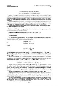
As an example, suppose each of the Ak's and C has block structure as shown in Figure 1; then we have blk{l, 1) = 'nondiag' blk{2,1) = 'nondiag' blk{3,1) = 'diag'

blk{1,2) = 50 blk{2,2) = [5 5 . . . 51 blk{3,2) = 100

and the matrices Ak and C are stored in cell arrays as A{i,k), A{2, k) , A{3,k),

C{i) C{2) C{3)

[50x50 doublel = [SO0 x 500 sparse] = [100x 1 double] =

Notice that when the block is a diagonal matrix, only the diagonal elements are stored, and they are stored as a column vector. Recall that when a block is a sparse block-diagonal matrix consisting of t sub-blocks of dimensions nil),n?), . . . , nf), we can actually view it as t individual blocks, in which case there will be t cell array elements associated with the t blocks rather than just one single cell array element originally associated with the sparse block-diagonal matrix. The reason for using the sparse matrix representation to handle the case when we have numerous small diagonal blocks is that it is less efficient for MATLAB to work with a large number of cell array elements compared to working

SDPT3-MATLABSOFTWARE PACKAGE

1oox 100

FIGURE 1 An example of a block-diagonal matrix.

with a single cell array element consisting of a large sparse block-diagonal matrix. Technically, no problem will arise if one chooses to store the small blocks individually instead of grouping them together as a sparse block-diagonal matrix. We should also mention the function file 0ps.m used in our package. The purpose of this file is to facilitate arithmetic operations on the contents of any two cell arrays with constituents that are matrices of corresponding dimensions. cell arrays, we refer to [14]. For the usage of MATLAB

Complex data Complex SDP data are allowed in our package. The user does not have to make any declaration even when the data is complex. Our codes will automatically detect whether this is the case.

Caveats The user should be aware that semidefinite programming is more complicated than linear programming. For example, it is possible that

K. C. TOH et al.

570

both primal and dual problems are feasible, but their optimal values are not equal. Also, either problem may be infeasible without there being a certificate of that fact (so-called weak infeasibility). In such cases, our software package is likely to terminate after some iterations with an indication of short step-length or lack of progress. Also, even if there is a certificate of infeasibility, our infeasible-interior-point methods may not find it. Our homogeneous self-dual methods may also fail to detect infeasibility, but they are practical variants of theoretical methods that are guaranteed to obtain certificates of infeasibility if such exist. In our very limited testing on strongly infeasible problems, most of our algorithms have been quite successful in detecting infeasibility.

6 EXAMPLE FILES

To solve a given SDP, the user needs to express it in the standard form (1) and (2), and then write a function file, say problem.m,to compute the input data blk,A,C, b,XO,yo,ZO for the solvers sdp.m or sdphlf .m.This function file may take the form [blk,A,C,b,XO,yo,ZO] = problem(input arguments)

Alternatively, one can provide the data in the input format described in [ 5 ] ,which is based on that of [9], and execute the function (based on a routine written by Brian Borchers) [blk,A,C,b,XO,yo,ZO] = read-sdpa('f ilename').

The user can easily learn how to use this software package by reading the script file demo.m, which illustrates how the solvers sdp.m and sdphlf .m can be used to solve a few SDP examples. The next section shows how sdp.m and sdphlf .m can be used to solve random problems generated by randsdp.m,graph.m,and maxcut.m,and the resulting output, for several of our algorithms. This software package also includes example files for the following classes of SDPs. In these files, unless otherwise stated, the input variables feas and solve are used as follows: f eas =

corresponds to the initial iterate given in (42), 1 corresponds to a feasible initial iterate;

0

SDPT3-MATLABSOFTWARE PACKAGE

0 only gives the input data blk, A, C, b,XO, yo, ZO for sdp. m, or sdphlf. m, solve = 1 solves the given problem by an infeasible path-following algorithm, 2 solves the given problem by , a homogeneous self-dual algorithm. If solve is positive, the output variable objval is the objective value of the associated optimization problem, and the output variables after ob jval give approximately optimal solutions to the original problem and its dual (or possibly indications of infeasibility). Here are our examples. (1) Random SDP: The associated M-file is randsdp.m, with initial line [blk,A,C,b,XO,yO,ZO,objval,X,y,Z] = randsdp (de,sp,di ,m,feas, solve), where the input parameters describe a particular block diagonal structure for each Ak and C . Specifically, the vector de is a list of dimensions of dense blocks; the vector sp is a list of dimensions of (small) subblocks in a single sparse block; and the scalar di is the size of the diagonal block. The scalar m is the number of equality constraints. There is an alternative function randinf sdp.m that generates primal or dual infeasible problems. The associated M-file has the initial line [blk,A,C,b,XO,yO,ZO,objval,X,y,Z] = randinfsdp (de,sp,di,m,infeas,solve).

The input variables de,sp,di, and solve all have the same meaning as in randsdp.m,but the variable inf eas is used as follows: inf eas =

1 if want primal infeasible pair of problems,

2

if want dual infeasible pair of problems.

(2) Norm minimization problem [23]:

where the B k , k = 0, . . . , m, are p x q matrices (possibly complex, in and the norm is the matrix 2-norm. which case x ranges over

em)

572

K. C. TOH et al.

.

The associated M-file is norm-min m, with initial line [blk,A,C,b,XO,yo, ZO,objval ,XI norm-min (B,f eas ,solve) ,

=

where B is a cell array with B{k + 1) = Bk,k = 0,. . . ,m. (3) Chebyshev approximation problem for a matrix [22]:

where the minimization is over the class of monic polynomials of degree m, B is a square matrix (possibly complex) and the norm is the matrix 2-norm. The associated M-file is chebyrnat.m,with initial line [blk,A,C, b,XO, yo ,ZO,objval ,p] chebymat (B,m,feas,solve).

=

See also igmres.m,which solves an analogous problem with p normalized such that p(0) = 1. (4) Max-Cut problem [lo]:

where L = B - Diag(Be), e is the vector of all ones and B is the weighted adjacency matrix of a graph [lo]. The associated M-file is maxcut.m, with initial line [blk,A,C,b,XO,yO,ZO,objval,XI maxcut (B, f eas ,solve) .

=

See also graph.m, from which the user can generate a weighted adjacency matrix B of a random graph. (5) ETP (Educational testing problem) [23]:

where B is a real N x N positive definite matrix and e is again the vector of all ones. The associated M-file is etp.m, with initial line [blk,A,C,b ,XO,y0,ZO, objval ,dl etp (B , f eas ,solve)

=

.

SDPT~-MATLAB SOFTWARE PACKAGE

(6) Lovhsz 9 function for a graph [2]:

where C is the matrix of all minus ones, Al = I, and Ak = eie; + ejeT, where the (k - 1)st edge of the given graph (with m - 1 edges) is from vertex i to vertex j. Here ei denotes the ith unit vector. The associated M-file is theta.m. with initial line [blk,~,C,b,XO,yO,ZO,~bj~al,Xl theta (B,f eas, solve) ,

=

where B is the adjacency matrix of the graph. (7) Logarithmic Chebyshev approximation problem [23]:

where B = [blb2 . . . bNIT is a real N x m matrix and f is a real N vector. The associated M-file is 10gcheby.m~ with initial line [blk,A,C, b,XO, yO,ZO, objval ,XI = logcheby (B,f,feas,solve).

(8) Chebyshev approximation problem in the complex plane [22]:

where the minimization is over the class of monic polynomials of degree m and { d l , . . . , d ~ is) a given set of points in the complex plane. The associated M-file is chebyinf .m,with initial line [blk,A,C,b,XO,yo, ZO, objval ,pl chebyinf (d,m,feas,solve),

=

where d = [did2.. . dN]. See also chebyO.m,which solves an analogous problem with p normalized such that p(0) = 1.

K. C. TOH et al.

574

(9) Control and system problem [23]: maxt,pt

k t I , I P P = pT, Bk, k = 1,. . . , L, are square real matrices P

where of the same dimension. The associated M-file is control.m,with initial line [blk,A,C,b,XO,yO,ZO,objval,Pl = control (B,solve) , where B is a cell array with B{k) = Bk,k = I , . . . , L.

7 SAMPLE RUNS >> randn('seed' ,0) %reset random generator to its initla1 seed. >> rand('seed' ,0) % >> startup % set up default parameters in the OPTIONS structure, >> % set paths >> >> %'777Lrandom SDP %'/)I77/, >> >> de = [201 ; sp = [I ; di = [I ; % one 20x20 dense block, no sparse/diag blocks >> m = 20; X 20 equality constraints % feasible initial iterate >>feas= 1; % do not solve the problem, just generate data. >> solve = 0; >> Cblk,A,C,b,XO,yO,ZOl = randsdp(de,sp,di,m,feas,solve); >> >> 0PTIONS.gaptol = le - 12; %use a non-default relative accuracy tolerance % use AH0 direction >> 0PTIONS.vers = 1; >> % solve using IPC >> [obj,X,y,Z,gaphist,infeashistl = sdp(blk,A,C,b.XO.yO,ZO,OPTIONS); condition no. of A = 1.75 e t 00

....................................................................................... Infeasible path-following algorithms

....................................................................................... version predcorr gam expon use-corrprlm 1 1 0.0003 1 it pstep dstep p-infeas d-infeas gap

.

.

sv2PC-to1 Inf obj

pathres

sigma rcond

.

11 0.989 0.989 3.0e-14 7.8e-17 5.3e-09 -1.058223et03 6.9e-01 12 0.987 0.988 2.0e-14 7.5e-17 6.9e-11 -1.0582238+03 7.h-01 Stop: max(re1ative gap, infeasibilities) < 1.00e-12 number of iterations = 12 gap = 6.92e-11 = 6.54e-14 relative gap = 2.05e-14 infeasibilities = 3.7 Total CPU time CPU time per iteration = 0.3 0 termination code

-

0.000 1.9e-12 0.000 2.4e-14

S D ~ ~ - M A T LSOFTWARE AB PACKAGE

An explanation for the notations used in the iteration output above is in order: it : the iteration number. p s t e p , d s t e p : denote the step-lengths a and 3, respectively. p- i n f e a s , d- i n f e a s : denote the relative primal infeasibility r p / / ( l + lib/) and dual infeasibility R d F / ( l+ CllF),respectively. gap: the duality gap X 8 Z. o b j : the mean objective value (C X + b T y ) / 2 . p a t h r e s : the centrality measure 1 - X,,,(XZ)/p. sigma: the value used for the centering parameter o. rcond: the reciprocal of the condition number of the Schur complement matrix M in (10).

>> >> >> >> >> >> >> >>

% n e x t , g e n e r a t e new d a t a w i t h a d i f f e r e n t block s t r u c t u r e f e a s = 0 ; % and u s e t h e ( i n f e a s i b l e ) i n i t i a l i t e r a t e g i v e n i n (42) [blk,A,C,b,XO,yO,ZO] = randsdp ([20 151, [4 3 31,5.30, f e a s , s o l v e ) ; % u s e CT d i r e c t i o n % s o l v e u s i n g HPC [obj,X,y,Z,tau,kap,gaphist,infeashistl

0PTIONS.vers

**r rr*

= 4;

=

sdphlf (blk,A,C,b,XO,yO,Z0,1,1,OPTIONS);

not a d v i s a b l e t o c o r r e c t p r i m a l i n f e a s i b i l i t y i n homogeneous a l g o r i t h m s : s e t t i n g u s e - c o r r p r i m - 0

***********++******************+++++++*******************+**+++*********************++* Homogeneous s e l f - d u a l a l g o r i t h m s

....................................................................................... version 4

predcorr 1

gam expon 0.0002

it p s t e p d s t e p p - i n f e a s

use-corrprim 0

d-infeas

sv2PC-to1 Inf

gap

obj

pathres

S t o p : schurmatrixistooill-conditioned f o r f u r t h e r p r o g r e s s number of i t e r a t i o n s

= 16

-

1.90e-10 gap r e l a t i v e gap = 5.608-13 infeasibilities = 2.618-12 = 13.7 T o t a l CPU t i m e CPU t i m e p e r i t e r a t i o n 0 . 9 -5 t e r m i n a t i o n code

--

>> >> >> >> >> >> >> >> >> >> >> >>

%%'W MAXCUT PROBLEM %'/.%%% B = graph(50.0.3) ; % g e n e r a t e an adjacency m a t r i x of a 50 node graph % where each edge i s p r e s e n t w i t h p r o b a b i l i t y 0 . 3 f e a s = 1 ; % u s ea f e a s i b l e i n i t i a l i t e r a t e ; s o l v e = 1 ; % g e n e r a t e d a t a , t h e n s o l v e t h e problem u s i n g IPC ' / . w i t h d e f a u l t parameters s e t up f o r t h e OPTIONS s t r u c t u r e % i n paramters .m % next s o l v e t h e maxcut problem d e f i n e d on t h e g i v e n graph

[blk,A,C,b,XO,yO,ZO,objval,Xl -maxcut ( B , f e a s , s o l v e ) ;

sigma rcond

K.C. TOH et al.

576

....................................................................................... I n f e a s i b l e path-following algorithms

....................................................................................... version 3

predcorr 1

gam 0.000

it p s t e p d s t e p p - i n f e a s

expon

use-corrprim

1

d-infeas

1

gap

sw2PC-to1 Inf obj

pathres

sigma rcond

S t o p : m a x b l a t i v s gap, i n f e a s i b i l i t i e s ) < 1.00e-08 number of i t e r a t i o n s

--

= 10

2.83~-07 gap 1.12e-09 r e l a t i v e gap infeasibilities -4.81e-17 T o t a l CPU t i m e = 5.4 CPU t i m e p e r i t e r a t i o n = 0 . 5 = 0 t e r m i n a t i o n code

8 NUMERICAL RESULTS The tables below show the performance of the algorithms discussed in Section 2 and 3 on the first eight SDP examples described in Section 6. The result for each example is based on ten random instances with command randn.The normally distributed data generated via the MATLAB initial iterate for each problem is infeasible, generated from inf easpt.m with the default option. Note that the same set of random instances is used throughout for each example. In Tables I1 and 111, we use the default value (given in Section 5) for the parameters used in the algorithms, except for OPTIONS.gapto1, which is set to l e - 13. In our experiments, let us call an SDP instance successfully solved by Algorithm IPC if the algorithm manages to reduce the relative duality gap X Z/(1 + ltC X I ) to less than lop6 while at the same time the infeasibility measure 4 is less than the relative duality gap. For Algorithm HPC, we call an SDP instance successfully solved if the relative duality gap is less than loF6 while the infeasibility measure 4 is at most 5 times more than the relative duality gap. We do not terminate the algorithms when this measure of success is attained. All of the SDP instances (a total of 640) considered in our experiments were successfully solved, except for only three ETP instances and one

SDPT3-MATLABSOFTWARE PACKAGE

577

Logarithmic Chebyshev instance where Algorithm HPC using the AH0 direction failed. This indicates that our algorithms are probably quite robust. The results in Tables I1 and I11 show that the behavior of Algorithms IPC and HPC are quite similar in terms of efficiency (as measured by the number of iterations) and accuracy on all the the four search directions we implemented. Note that we give the number of iterations and the CPU time required to reduce the duality gap by a factor of 10'' compared to its original value (the relative gap may then be still too large to conclude "success"), and also the minimum relative gap achieved by each method. For both algorithms, the AH0 and GT directions are more TABLE I1 Computational results on different classes of SDP for Algorithm IPC. Ten random instances are considered for each class. The computations were done on a DEC AlphaStation.600 (333MHz). The number X Z above is the smallest number such that and the infeasibility measure C$ is relative duality gap X * Z/(1 + IC* XI) is less than less than the relative duality gap Algorithm IPC

Ave. no. of iterations Ave. CPU time (sec.) to reduce the duality to reduce the duality gap by 10l0 gap by 10l0

Accuracy mean ( loglo(X 21)

AH0 GT HKM NT AH0 GT HKM NT AH0 GT HKM NT random SDP Norm min. problem Cheby. approx. of a real matrix Maxcut ETP

function Log. Cheby. problem Cheby. approx. on C

n = 50 m = 50 n = 100 m = 26 n=100 m = 26 n = 50 m = 50 n=100

m

-

10.6 11.2 12.7 11.7 15.8 12.1 11.1 10.7 7.4 6.4

6.1

5.8

9.1 9.4 10.8 11.0 39.4 29.3 23.4 26.5 11.9 12.4

9.6

9.1

8.8 9.3 10.8 11.5 37.9 28.4 24.8 27.5 13.7 13.6 10.8 10.5

9.9 10.5 11.5 11.7 11.3 7.9

5.8

6.2 10.9 9.8

9.0

8.7

17.1 17.5 20.3 19.9 25.6 17.3 14.2 14.4 8.8 8.8

7.1

7.2

12.6 13.0 13.7 13.7 24.6 21.2 15.2 18.2 9.6

9.7

9.8

220

n = 300 m = 51 n=200 m=41

9.7

9.9 10.2 11.1 11.3 15.7 14.4 11.0 13.6 12.9 13.0 10.9 10.9

K. C. TOH et al.

578

efficient and more accurate than the HKM and NT directions, with the former and latter pairs having similar behavior in terms of efficiency and accuracy. Efficiency can alternatively be measured by the total CPU time required. The performances of Algorithms IPC and HPC are also quite similar in terms of the CPU time taken to reduce the duality gap by a prescribed factor on all the four directions. But in this case, the NT and HKM directions are the fastest, followed by the GT direction which is about 20% to 30% slower, and the A H 0 direction is the slowest where it is usually at least about 60% slower.

.

TABLE 111 Same as Table 11, but for the homogenous predictor-corrector algorithm, Algorithm HPC. The duality gapX Z above is the smallest number such that the relative duality gap X Z/(1 + IC XI) is less than 10@ and the infeasibility measure q5 is at most 5 times more than the relative duality gap

.

Algorithm HPC

.

Accuracy Ave. no. of iterations Ave. CPU time (sec.) to reduce the duality to reduce the duality mean(1 loglo(X Z)I) gap by 10l0 gap by 101° A H 0 GT HKM NT A H 0 GT HKM NT A H 0 GT HKM NT

random SDP Norm min. problem Cheby. approx. of a real matrix Maxcut

n = 50 m = 50 n = 100 m = 26 n=100 m = 26 n = 50

10.4 10.9 11.4 11.0 15.7 11.7 9.7

6.4

6.0

10.9 10.2 11.9 11.5 48.7 32.3 25.8 27.7 11.1 11.5 9.6

9.0

8.8 8.1

10.1 10.1 11.8 11.1 44.4 31.6 26.9 26.4 13.7 12.8 11.1 10.5

9.9 9.7 11.1 10.6 11.8 7.6

n = 1 0 0 14.3*15.3 17.1 16.6 m = 50 Lov6szO n=30 11.5 11.7 12.9 12.8 function m = 220 Log. Cheby. n = 300 15.0*12.5 13.2 13.2 problem m = 51 Cheby. n=200 9.8 9.6 10.1 10.0 approx. on @ m = 41 ETP

9.7

213'15.5

5.8

5.8 10.8 10.1

9.2

8.6

12.1 12.1 9.4' 9.5

7.2

6.9

44.6 29.8 24.8 22.4 12.2 11.5 11.0 10.5 31.7* 21.3 15.4 18.4 12.2*12.9 12.4 12.4

16.5 14.5 10.1 12.5 13.5 13.3 11.5 11.5

'Three of the ETP instances fail because the infeasibility measure 4 is consistently 5 times more than the One of the Log. relative duality gap X Z/(1+ /C* XI)when the relative duality gap is less than Cheby. instances fails due to step lengths going below The numbers reported here are based on the successful instances.

SDPT~-MATLAB SOFTWARE PACKAGE

579

Finally, to give the reader an idea of the amount of CPU time spent in various steps of our algorithms, we give the breakdowns of the CPU time spent in algorithm IPC with GT direction on a random SDP problem with n, m = 100. This is done using the MATLAB command profile.

>> >> >> >>

[blk,A,C,b ,XO ,yo,ZOI = randsdp (100,[I , [I ,100); profile sdp sdp (blk,A,C,b,XO,yO,ZO,OPTIONS); profile report 5 Total time in ll./Solver/sdp.mll: 184.65 seconds 91% of the total time was spent on lines: 81% 2% 4% 2% 2%

252: 277: 342: 356: 418:

GTpred.m c0rrprim.m GTcorr .m c0rrprim.m ZpATy=ops(Z, '+',Asum(A,y));

>> >> profile GTpred >> sdp ~ ~ ~ ~ , A , C , ~ , X O , ~ O , Z O , O; P T I O N S ~ >> profile report 5 Total time in I1./Solver/GTpred.m":154.59 seconds 86% of the total time was spent on lines 2% 21% 37%

34: 35: 36:

26%

43:

tmp = XR {P) (:,PA {p,k)); tmp = Prod2 (tmp,LA {p,k),22) ; tmp = Prod3 (tmp,TA {p,k),ops (tmp,'ctranspose') ,I); schur-tmp (l:k,k) = blktrace (B(p,l:k) ,tmp);

The last four lines correspond to the formation of the Schur complement matrix M in the predictor step. Evidently, it is the most expensive step of the algorithm in which about 80% of the total CPU time is spent.

Acknowledgments The authors thank Christoph Helmberg for many constructive suggestions.

580

K. C. TOH et al.

References [I] Aasen, J. 0. (1971). On the reduction of a symmetric matrix to tridiagonal form, BIT 11, 233-242. [2] Alizadeh, F. (1995). Interior point methods in semidefinite programming with applications to combinatorial optimization, SIAM J. Optimization, 5, 13-51. [3] Alizadeh, F., Haeberly, J. -P. A. and Overton, M. L. (1998). Primal-dual interior-point methods for semidefinite programming: convergence results, stability and numerical results, SIAM J. Optimization, 8, 746-768. [4] Alizadeh, F., Haeberly, J. -P. A., Nayakkankuppam, M. V., Overton, M. L. and Schmieta, S. SDPPACK user's guide, Technical Report, Computer Science Department, NYU, New York, June 1997. [5] Borchers, B. SDPLIB, A Library of Semidejnite Programming Test Problems, available fromhttp://www.nmt.edu/borchers/sdplib.html. [6] Brixius, N., Potra, F. A. and Sheng, R. (1996). Solving semidejinite programming in Mathernatica, Reports on Computational Mathematics, No 9711996, Department of Mathematics, University of Iowa, October. Available at http://www.cs.uiowa.edu/brixius/sdp.html. [7] Brixius, N., Potra, F. A. and Sheng, R. (1998). SDPHA: A Matlab implementation of homogeneous interior-point algorithms for semidejinite programming, available from h t t p : //www. c s .uiowa. edu/'brixius/SDPHA/, May. [8] Fujisawa, K., Kojima, M. and Nakata, K. (1997). Exploiting sparsity in primal-dual interior-point method for semidefinite programming, Mathematical Programming, 79, 235-253. [9] Fujisawa, K., Kojima, M. and Nakata, K. SDPA (semidejnite programming algorithm) - user's manual, Research Report, Department of Mathematical and Computing Science, Tokyo Institute of Technology, Tokyo. Available via anonymous ftp at f t p . i s . t i t e c h . a c . j p inpub/OpRes/software/SDPA. [lo] Helmberg, C., Rendl, F., Vanderbei R. and Wolkowicz, H. (1996). An interior-point method for semidefinite programming, SIAM Journal on Optimization, 6 , 342-361. [ l l ] de Klerk, E., Roos, C. and Terlaky, T. (1997). Infeasible start, semidejinite programming algorithms via self-dual embeddings, Report 97-10, TWI, Delft University of ~ e c h n o l o April. ~~, [12] Kojima, M., Shindoh, S. and Hara, S. (1997). Interior-point methods for the monotone linear complementarity problem in symmetric matrices, SIAM J. Optimization, 7, 86-125. [13] Luo, 2. -Q., Sturm, J. F. and Zhang, S. (1996). Duality and self-dualityfor conic convex programming, Technical Report 9620/A, Tinbergen Institute, Erasmus University, Rotterdam. [14] The Math Works, Inc., Using MATUB, The Math Works, Inc., Natick, MA, 1997. [I51 Mehrotra, S. (1992). On the implementation of a primal-dual interior point method, SIAM J. Optimization, 2, 575-601. [16] Monteiro, R. D. C. (1997). Primal-Dual Path-Following Algorithms for Semidefinite Programming, SIAM J. Optimization, 7, 663-678. [17] Potra, F. A, and Sheng, R. (1998). On homogeneous interior-point algorithms for semidefinite programming, Optimization Methods and Software 9, 161- 184. [18] Saad, Y. Iterative Methods for Sparse Linear Systems, PWS Publishing Company, Boston. [19] Sturm, J. F. (1998). SeDuMi 1.00: Self-dual-minimization Matlab 5 toolbox for optimization over symmetric cones, Communications Research Laboratory, McMaster University, Hamilton, Canada, April. [20] Todd, M. J.. Toh, K. C. and Tiitiincu, R. H. (1998). On the Nesterov-Todd direction in semidefinite programming, SIAM J. Optimization, 8, 769-796. [21] Toh, K. C. (1998). Search directions forprimal-dual interior point methods in semidefinite programming, Technical Report No. 722, Department of Mathematics, National University of Singapore, Singapore, July, 1997. Revised in March.

SDPT3-MATLABSOFTWARE PACKAGE

581

[22] Toh, K. C. and Trefethen, L. N. The Chebyshev polynomials of a matrix, to appear in SIAM J. Matrix Analysis and Applications. [23] Vandenberghe, L. and Boyd, S. (1996). Semidefinite programming, SIAM Review, 38, 49-95. [24] Vandenberghe, L. and Boyd, S. (1994). User's guide to SP: software for semidefinite programming, Information Systems Laboratory, Stanford University, November 1994. Available via anonymous ftp at is1 . stanf ord. edu in pub/boyd/semidef -prog. Beta version. [25] Xu, X., Hung, P. -F. and Ye, Y. (1996). A simplified homogeneous and self-dual linear programming algorithm and its implementation, Annals of Operations Research, 62, 151-171 -- - - . - . [26] Ye, Y., Todd, M. J. and Mizuno, S. (1994). An O(JnL)-iteration homogeneous and self-dual linear programming algorithm, Mathematics of Operations Research, 19, 53-67.