Searching and Mapping among Indistinguishable Convex Obstacles

Searching and Mapping among Indistinguishable Convex Obstacles Benjamin Tovar and Steven M. LaValle

Abstract— We present exploration and mapping strategies for a mobile robot moving among a finite collection of convex obstacles in the plane. The obstacles are unknown to the robot, which does not have access to coordinates and cannot measure distances or angles. The robot has a unique sensor, called the gap sensor, that tracks the direction of the depth discontinuities in the robot’s visibility region. Furthermore, the robot can only move towards depth discontinuities. As the robot moves, the depth discontinuities split and merge, and these changes are encoded in a Gap Navigation Tree. We present a strategy for this robot that is guaranteed to explore the whole environment, but that cannot decide whether the exploration has been completed. If in addition it is assumed that the robot has access to a pebble, which is an identifiable point that the robot can manipulate, then we prove that the robot can decide (in polynomial time in the number of obstacles) whether the environment has been completely explored. For this, the robot is able to distinguish every obstacle using only the gap sensor and a single pebble. These results are a continuation of our previous work on gap sensing for multiply connected environments [24], in which we reduce the sensing requirements for the robot by constraining the shape of the obstacles.

I. I NTRODUCTION These paper focuses on developing systematic exploration strategies for robots moving in unknown environments [4], [9], [10]. This is inspired from the lost-cow problem, in which a cow moves along a fence trying to find a gate to access a pasture. The cow does not know where the entrance is, or how far it could be. A solution to the lost cow problem is a strategy for the cow that guarantees it will find the gate. This problem is usually modeled by considering the fence as the integer line, with the cow starting at the origin, and the gate positioned at some number d, unknown to the cow. Consider the strategy in which at each stage i, the cow walks 2i steps in one direction, comes back to the origin, walks 2i steps in the opposite direction, and finally comes back to the origin. In the worst case, the cow takes 9d steps, and this in fact minimizes the worst case distance traveled by the cow [1]. Note that the cow cannot determine the absence of a gate in the fence. In such a case, no cow strategy terminates, as the search for the gate continues forever. In our case, the “cow” is a robot moving in the plane, the “fence” is a finite collection of indistinguishable convex obstacles, and the “gate” becomes a treasure, which is an identifiable point in the environment, recognized as soon as it enters the robot’s omnidirectional and unbounded field of view. Here we assume that the robot has an abstract B. Tovar is with the Department of Mechanical Engineering, Northwestern University, 2145 Sheridan Road, Evanston, IL 60208, USA.

[email protected] S. M. LaValle is with the Department of Computer Science, University of Illinois, Urbana, IL 45435, USA. [email protected]

sensor [7] that reports the order of depth discontinuities in the robot’s visibility region. These depth discontinuities are characterized by the obstacle they start at from the robot perspective, and by the side to which they hide the environment to the robot. Two discontinuities with the same origin and side are considered equivalent, and the equivalence classes are called gaps. To characterize its environment, the robot builds a dynamic data structure, called the Gap Navigation Tree (GNT), entirely from online sensor measurements. Once constructed, it encodes paths from the current position of the robot to any place in the environment [24]. Can convex obstacles be distinguished with only gap sensing? In Section III we present a strategy that systematically explore the environment reachable by the robot, using uniquely a gap sensor. Even though this strategy guarantees that all of the environment is eventually explored, it does not terminate. In Section IV, we further assume that the robot has access to one pebble, which is a special point that can be detected and moved by the robot. We prove that with the pebble, the robot can decide, in polynomial time, whether the environment has been completely explored. This is done by distinguishing obstacles using only the gap sensor and a single pebble. This work is a continuation of our study of minimal robot models by sensing gaps. In [24] we presented an exploration strategy for multiply connected environments assuming the robot could distinguish among the obstacles. In this paper we remove this assumption, but constrain the obstacles to be convex. This constrain is only necessary for deciding whether the environment has been completely explored, since a systematic search of the environment is still possible among non-convex obstacles. Our work is inspired by minimal sensing for mobile robots from works such as bug algorithms [11], [12], [13], [16], [17], in which a robot that combines global knowledge with local information is able to navigate among boundary components and reach a known goal. In the case of bug algorithms, the robot navigation capabilities are simple (movement towards boundary components and wall-following), no representation of the environment is maintained, and the global information consists only of the position of the goal. These characteristics allow the use of bug algorithms in robots that have very limited sensing capabilities and unreliable motion control. More importantly, the memory required for the algorithms is constant. Such online exploration strategies make simple motion models and attempt to reduce the amount of memory or total distance traveled [3], [5], [6], [8], [9], [14], [15], [18], [19], [23].

II. BASIC D EFINITIONS Let O be a nonempty finite collection of pairwise-disjoint sets in the plane R2 , called the obstacles. Each O ∈ O is compact (i.e., closed and bounded), and convex, meaning that the closed line segment joining any two points in O does not intersect R2 \O. Furthermore, it is assumed that the boundary ∂O of each O ∈ O is piecewise-analytic. Let F , the free space, be the closure of R2 \ O (i.e., the plane minus the interior of the obstacles). We model the robot’s configurations as the set X = F × S 1 ⊆ SE(2). Observe that F includes the boundary of the obstacles, therefore, the robot can execute compliant motions (i.e., in contact) with the obstacles. For q ∈ F , let V (q) be the visibility region of q, in which p ∈ V (q) if and only if the closed line segment joining p and q does not intersect R2 \ O. The visibility region consists of three kinds of segments: 1) Curve segments completely contained in ∂F . 2) Compact line segments collinear with q, and which intersect ∂F only at their endpoints, both of which belong to ∂F . 3) Half-lines collinear with q, which intersect ∂F only at their unique endpoint. Segments of the second and third kind are called depth discontinuities. If a depth discontinuity d is a half-line, define the origin of d, o(d), as the obstacle O ∈ O that contains the endpoint of d in its boundary. Otherwise, if a depth discontinuity d has two endpoints, define o(d) as the obstacle O ∈ O that contains the endpoint of d closer to q in its boundary. Each depth discontinuity d is directed, and starts from the point in o(d). Every depth discontinuity d receives a label s(d) of left or right, depending on which side of d F \ V (q) is, as seen from q. If depth discontinuities are reported counterclockwise from a visibility region, then the left label corresponds to a transition from far to near, and the right label corresponds to a transition from near to far [24]. This label also corresponds to the side of the depth discontinuities on which the obstacle appears, as seen from q. Now we define gaps in terms of depth discontinuities: Definition 1: Two depth discontinuities di and dj are said to be equivalent if o(di ) = o(dj ) and s(di ) = s(dj ). The equivalence classes of depth discontinuities are called gaps. We cannot use Definition 1 for gaps with non-convex obstacles. This is because with non-convex obstacles, distinct gaps may share the same origin, and have the same side label. Every obstacle O ∈ O is the origin of exactly two gaps, one labeled right, and the other labeled left. We say that these two gaps are associated with obstacle O. Let r(O) and l(O) be the gaps associated with O, with side label right and left respectively. Sensor: We consider a robot which is not able to compute V (q), but that instead has a gap sensor, which is able to track the gaps in V (q) at all times, reports them in their counterclockwise cyclic order as they appear in V (q), and determines their side labels. Note that the gaps’s size, angle, origin, and distance to the robot are not reported by

the gap sensor. Motion primitive: The robot moves by chasing gaps. To chase a gap, the robot orients its heading with the gap, and moves towards it. A. The Gap Navigation Tree Here we give a brief description of the Gap Navigation Tree data structure. For the complete description please refer to [24]. In a Gap Navigation Tree, the root represents the gap sensor, and each vertex represents a gap. Children of the root represent gaps currently detected, and are maintained in the cyclic order in which they appear in the gap sensor. As the robot moves in F , V (q) changes combinatorially. In particular, the number of gaps in ∂V (q) may decrease or increase through the following critical events: • Gaps merge. For gaps gi and gj assume that q is closer to o(gi ) than it is to o(gj ). If gj becomes collinear with gi , so that gj is no longer contained in ∂V (q), then we say that gj merged into gi . • Gaps split. Let gi and gj be two gaps, so that gj became part of ∂V (q) by first being collinear with gi . We say that gi split, or that gj split from gi . Note that since every O ∈ O is compact and convex, gaps may only split or merge, but they cannot appear or disappear. If a gap splits, then the corresponding child of the root is replaced with two children. When two gaps merge, the two corresponding children of the root become the children of a new vertex, and this new vertex becomes a child of the root. A sequence of vertices from the root to a leaf define a sequence of gaps, that if chased, follows a path in the shortest-path graph of F . III. S YSTEMATICALLY E XPLORING

THE

E NVIRONMENT

Now we develop a strategy with the guarantee that every point in F appears eventually in the visibility region of the robot. To present the strategy, we define a special point in F , called the treasure, and show that independently of which point of F is defined to be the treasure, the robot will eventually see it. Strategy 1: Looking for a treasure among indistinguishable convex obstacles with a gap sensor Description: We construct a GNT according to the updates in Section II-A. Additionally, the leaves of the tree are labeled according to a counter, i. We call this label the exploration label of the vertex. The exploration labels of the m vertices corresponding to the initial m gaps observed are set 1 trough m, and i is set to m + 1. The search for the treasure proceeds by systematically chasing the gap g corresponding to the leaf with the minimum exploration label. Gap g is chased until its descendants are not known (that is, until the corresponding leaf in the tree splits). In this case, two new vertices are added to the root of the GNT, one corresponding to g, and the other to the gap, g ′ , that split from g. These two new vertices are labeled i and i + 1, respectively, and i is set to i + 2 (see Figure 1). Note that when two gaps merge, the internal vertex created is never

labeled for future exploration. If at any point the treasure becomes visible, then the strategy successfully terminates. Theorem 1: If there is a treasure, Strategy 1 is guaranteed to find it. Proof: Assume that from the initial position of the robot, the treasure is found by following the shortest sequence of gaps [g1 , g2 , . . . , gk ]. Initially, for j = 1, gj is visible, and therefore its vertex is labeled for exploration. Recursively, when gj is chased, gj+1 will split from it, and the corresponding vertices are labeled for future exploration. Eventually, gk is chased and the treasure is found. Note that Strategy 1 is easily extended to non-convex obstacles. In such a case, gaps are chased until they split or disappear, and the leaves corresponding to gap appearances do not need to be labeled according to the counter. Strategy 1 is terribly inefficient. Gaps are chased over and over again, as exemplified in Figure 1. Suppose that from the initial position of the robot, the shortest sequence of chase(·) motion primitives that finds the treasure has length k. Strategy 1 is a breadth-first search, in which each node has a branching factor of 2 (when a gap splits, two more nodes are added to the search queue, which is implemented through the exploration labels). Therefore, if it performs k chase(·) motion primitives in the optimal case, Strategy 1 performs O(2k ). Each vertex in the GNT corresponds to a bitangent complement [24] of F . Two vertices in the tree are said to be redundant if they correspond to the same bitangent complement. The issue here is that when a gap without known descendants splits, the newly created descendants may already be in some other branch of the tree. How can the robot detect redundant vertices? IV. D ISTINGUISHING O BSTACLES We define a left loop over obstacle O as the process of the robot reaching some point of ∂O, and chasing l(O) until ∂O is transversed exactly once. Similarly, a right loop over obstacle O is defined by chasing r(O). Consider the sequence of gap critical events as the robot performs a left loop on some obstacle O, and compare it to the sequence of gap critical events should the robot perform a right loop on that same obstacle. We should expect these sequences to be similar. To make this apparent, we define four stacks of gaps, merge(l(O)), merge(r(O)), split(l(O)), and split(r(O)), which are initially empty. When the robot performs a left loop over O, gaps merging with r(O) are pushed into merge(r(O)), and gaps splitting from l(O) are pushed into split(l(O)). The stacks merge(l(O)) and split(r(O)) are used similarly for a right loop over O. Lemma 2: For initially empty stacks merge(l(O)), merge(r(O)), split(r(O)), split(l(O)), after left and right loops, the sequence of gaps in merge(l(O) is the reversal up to a cyclic shift of the elements in merge(r(O)), and split(l(O)) is the reversal up to a cyclic shift of the elements in split(r(O)). Proof: Let p ∈ ∂O be the point at which the left loop over O starts, and let G(p) = [r(O), g1 , g2 , g3 , . . . , l(O)]

be the reading from the gap sensor at p. As the robot chases l(O), gaps that were not visible from p, g1′ , g2′ , g3′ , etc., split from l(O); the same will eventually happen with g1 , g2 , g3 , etc. When the robot reaches p, split(l(O)) = [. . . , g3 , g2 , g1 , . . . , g3′ , g2′ , g1′ ]. Similarly, while chasing l(O), gaps g1 , g2 , g3 , etc. merge (in that order) into r(O), as do the gaps not initially visible from p, g1′ , g2′ , g3′ , etc. At the end of the left loop over O, merge(r(O)) = [. . . , g3′ , g2′ , g1′ , . . . , g3 , g2 , g1 ]. Observe that split(l(O)) and merge(r(O)) are the same sequence up to a cyclic shift. Since split(r(O)) is the reversal of merge(r(O)), and merge(l(O)) is the reversal of split(l(O)), the result follows. Lemma 2 has important consequences for the structure of branches in a Gap Navigation Tree: Corollary 3: For O ∈ O, in a GNT without redundant vertices, after left and right loops over O, the first descendant of l(O) is the last descendant of r(O), and vice-versa. Proof: This is just an alternative wording of Lemma 2 in terms of the GNT structure. After a left loop over some obstacle, the length of merge(r(O)) determines the maximum number of merges of l(O) and r(O) without creating redundancies in the Gap Navigation Tree. After a left loop over O ∈ O, consider the branch starting at the root’s child associated with r(O). Observe that there is a sequence of m consecutive vertices which correspond to gaps merging into r(O). By Corollary 3, if more than m gaps merged into r(O), then the tree contains redundant vertices, and the branch can be pruned to the first m merges of r(O). Another consequence of Corollary 3 is that the branch for the root’s children associated with l(O) can be constructed from the branch of r(O), and vice-versa. Note that in addition to reversing the order of the merges, if a gap g merges to the left (resp. right) of r(O), then it merges to the right (resp. left) of l(O). Therefore, the branches corresponding to l(O) and r(O) can be compared, and completed or pruned accordingly. During the left and right loops over O, l(O) and r(O) appear consecutively in the sensor reading. With this observation, we can identify when two gaps have the same origin: Lemma 4: Let G(p) = [g1 , g2 , . . . , gn ] be the reading from the gap sensor from point p ∈ F . If s(gi ) = lef t and s(g1+(i mod n) ) = right, then o(gi ) = o(g1+(i mod n) ). Proof: Remember that the gap sensor detects gaps in a counterclockwise order. By assumption, there are no gaps between gi and g1+(i mod n) , which means either that the reading of the depth discontinuity sensor goes to infinity, or that the portion of ∂F detected does not have any discontinuities from the current point of view. The first case contradicts that the obstacle o(gi ) lies to the left of gi , and that obstacle o(g1+(i mod n) ) lies to the right of g1+(i mod n) . The second case implies that there is a connected portion of ∂F between gi and g1+(i mod n) . Therefore, o(gi ) = o(g1+(i mod n) ). Corollary 3 describes the structure of two branches when the robot is at the boundary of some obstacle. To use this result, the robot needs to perform left loops over the obstacles. However, this is not possible in general, since the robot cannot determine when it performed a complete loop

(a)

(b)

(c)

(d)

(e)

(f)

Fig. 1. Search for a treasure with Strategy 1. (a) The two vertices corresponding to the initially visible gaps are labeled for exploration, and the robot chases the gap associated with the minimum exploration label (label 1). (b) The gap being chased splits, and the new children are label consecutively for exploration, labels 3 and 4. The next gap chased corresponds to the vertex labeled 2. (c) Two leaves merge, and the resulting vertex is not labeled for exploration. (d) The gap being chased splits, with the children labeled for exploration with 5 and 6. (e) The gap associated with the vertex labeled 3 is chased, and the events are updated in the tree accordingly. (f) The gap being chased splits, with the children labeled 7 and 8. Note that the vertices labeled 5 and 8 are associated with the same gap, but such correspondence is not made by Strategy 1. The search continues by chasing the gap associated with the minimum exploration label.

around an obstacle. If we extend the robot model with a single pebble, which extra information can the robot determine? Can the robot distinguish the origin of all gaps using only the gap sensor and the pebble? Since the robot does not have a sensor that immediately identifies the obstacles, distinguishing obstacles means here that they are assigned arbitrary but consistent labels. With the addition of the pebble, the robot is provided with a new motion primitive, surround(O), which commands the robot to transverse completely the boundary of O ∈ O once. Consider the following strategy: Strategy 2: Looking for a treasure among indistinguishable obstacles with a gap sensor and a pebble Description: We keep two counters: counter i for the exploration labels, and counter j for naming obstacles. Both counters are initially set to 1. Observe that there are three cases for the information available regarding the origin of a gap g recorded in a vertex of the tree: 1) The origin of gap g is unknown. 2) The origin of gap g is unknown, but it can be determined it is the same origin as some other gap g ′ . 3) The origin of gap g is some obstacle Ok , for 1 ≤ k < j. The robot may not determine immediately that some gaps are associated with the same obstacle. Therefore, some obstacle may be labeled more than once. To handle this, the label for the origin of a gap is kept in the corresponding vertex of the tree. For exploration, the m gaps from the first observation are labeled 1 to m, and i is set to m + 1. Next, a GNT is constructed following the events in Section II-A, according to the following iteration: 1) Moving to an obstacle. Let g be the gap corresponding to the vertex in the GNT with minimum label for exploration. If no such gap exists, then the exploration is complete since F contains no treasure. Otherwise, the gap g is chased until the robot is in contact with

some obstacle O. 2) Labeling an obstacle. Since O was reached by chasing g, O is the origin of g, and g is one of l(O) or r(O). First, the exploration labels for the vertices of l(O) and r(O) are removed. Second, the origin in both vertices is set to Oj , and j is incremented. 3) Left loop over the obstacle. The robot drops the pebble, and performs a left loop over obstacle O. Every time l(O) splits without known descendants, the vertex corresponding to the gap splitting from l(O) is labeled i, and i is incremented. If a gap besides l(O) splits without known descendants, then the events of these descendants are ignored. They will eventually be labeled in a future iteration. 4) Modifying branches. The branches of the root’s children corresponding to l(O) and r(O) are compared and modified according to Corollary 3. The next iteration proceeds with step 1. If the treasure becomes visible at any point of the iteration, then the strategy terminates with success. An example of this strategy is shown in Figures 2 and 3. We discuss the correctness of Strategy 2: Theorem 5: If there is a treasure, strategy 2 is guaranteed to find it. Proof: Observe that the obstacles labels are a byproduct of Strategy 2, and do not determine the order in which gaps are explored. Suppose that Strategy 1 finds the treasure by chasing the sequence of gaps [g1 , g2 , . . . , gn ]. The vertex corresponding to g1 receives an exploration label in the initial step before the iteration. Recursively, starting with i = 1, a left loop is performed over o(gi ), from which gi+1 splits (Lemma 2), and its vertex is labeled for exploration. Eventually, a left loop is performed over o(gn ), which makes the treasure visible. We conjecture that the breadth-first search implemented by Strategy 2 labels each obstacle exactly once. Therefore, it would take at most O(|O|) iterations to find the treasure.

(a)

(b)

(c)

(d)

(e)

(f)

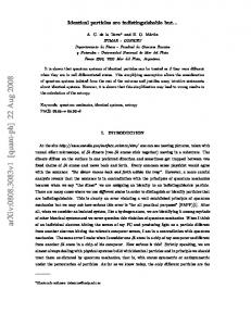
Fig. 2. Search for a treasure with Strategy 2 (I). For convenience, we will refer to l(Oj ) and r(Oj ), with l(j) and r(j), respectively. (a) The obstacle corresponding to the first boundary reached is labeled 1. The left and right gap of obstacle 1 are identified accordingly. A left loop over obstacle 1 is performed from (b) to (d). As l(1) splits, the vertices of the gaps that split from l(1) are labeled for exploration. (e) The left loop over obstacle 1 is completed, and the branch of l(1) is constructed according to Corollary 3. (f) The exploration continues chasing the gap associated with the vertex labeled 2 (continuation in Figure 3).

(a)

(b)

(c)

(d)

(e)

(f)

Fig. 3. Search for a treasure with Strategy 2 (II). Continuation of Figure 2. (a) When the new boundary is reached, the corresponding obstacle is labeled 2. From (b) to (d) a left loop over obstacle 2 is completed. For convenience, we only show the visible sections of the branches at (b). In (f), the branches are compared, and vertices labeled 4 and 5 are found to be l(1) and r(1) respectively. Also, the branch starting with l(2) is completed by mirroring the branch starting with r(2). At this point, no vertex remains labeled for exploration, and it is guaranteed that the environment did not contain a treasure.

More importantly, if every obstacle is labeled exactly once, Strategy 2 always terminates, as it does for the example presented in Figures 2 and 3. At the time of writing we do not have a prove to support these claims. However, with a small modification, Strategy 2 is guaranteed to label each obstacle exactly once, deciding the presence of a treasure in O(|O|3 ) time: Strategy 3: Looking for a treasure among indistinguishable obstacles with a gap sensor, a pebble, and backtracking Description: First, observe that once a left loop over some obstacle O ∈ O has been performed, a pebble is not needed anymore to implement the surround(O) motion primitive. By counting the number of gap critical events along ∂O, it can be guaranteed to be transversed exactly once. We modify Strategy 2 as follows. Assume that the label given to O ∈ O is j. Once the left loop is completed in step 3, the robot drops the pebble at Oj . For i = j − 1 down to 1, the robot chases back a gap with origin Oi , and performs surround(Oi ). If during surround(Oi ) the pebble is found, then Oi = Oj , the branches of the tree are matched accordingly, the counter j is decremented, and the iteration proceeds with step 1 of Strategy 2. Otherwise, if the pebble

is not found by surround(Oi ), Strategy 2 continues normally with step 4. This backtracking may avoid some unnecessary work. The surround(·) motion primitive should be performed only on obstacles with the same (cyclic) sequence of gap critical events along their boundary as the sequence for ∂Oj . Theorem 6: Strategy 3 decides in O(|O|3 ) time whether there is a treasure. Proof: An obstacle is only labeled with the current value of the counter if it is found not to be labeled before. Observe that for j > 1, surround(·) is performed j −1 times; if no obstacle is reached twice, then Strategy 3 terminates in Ω(|O|2 ) time. Otherwise, assume that for every O ∈ O, l(O) splits O(n) times. In the worst case, O(n) gaps that split from l(O) direct the robot to obstacles labeled before. This means that Strategy 3 terminates in O(|O|3 ) time. V. C ONCLUSIONS

AND

F UTURE W ORK

In this paper we presented exploration strategies for a mobile robot with limited sensing, moving among an unknown collection of convex obstacles. We proved that a robot with a gap sensor can systematically search the whole environment,

but it cannot decide whether every point of the free space has been visible. With the addition of a pebble, the robot can decide whether the environment has been completely explored. Assuming that the robot can distinguish among the collection of convex obstacles, the robot can recover the visibility type [20] of the collection of obstacles, which encodes all the information regarding critical changes in the visibility region of a moving point among the obstacles. The visibility type corresponds to cyclic sequences of bitangents along the boundary of the obstacles. The visibility type determines the tangent visibility graph [21], which is a generalization of the visibility graph for obstacles whose boundaries are not polygonal. In [20], based on the visibility type, pseudotriangulations are constructed. The sides of a pseudo-triangle are free bitangents and arcs on the boundary of the obstacles. Based on pseudo-triangulations, which are in fact oriented matroids of rank 3 ([2]), the visibility complex [22] can be constructed, allowing efficient visibility queries. Constructing the visibility complex from the information gathered by the robot described here seems feasible, and we consider it as future work. Acknowledgments.: The authors thank Lawrence Erickson for insightful discussions. Our work was partially funded by the DARPA SToMP Program. R EFERENCES [1] R.A. Baeza-Yates, J.C. Culberson, and G.J.E. Rawlins. Searching in the plane. Inf. Comput., 106(2):234–252, 1993. [2] A. Bj¨orner, M. Las Vergnas, B. Sturmfels, N. White, and G. M. Ziegler. Oriented matroids. Cambridge University Press, 1993. [3] A. Blum, P. Raghavan, and B. Schieber. Navigating in unfamiliar geometric terrains. In Proc. ACM Symp. Comp. Geom., pages 494– 504, 1991. [4] M. Blum and D. Kozen. On the power of the compass (or, why mazes are easier to search than graphs). In Proc. Annual Symposium on Foundations of Computer Science, pages 132–142, 1978. [5] A. Datta, C. A. Hipke, and S. Schuierer. Competitive searching in polygons–beyond generalized streets. In J. Staples, P. Eades, N. Katoh, and A. Moffat, editors, Algorithms and Computation, ISAAC ’95, pages 32–41. Springer-Verlag, Berlin, 1995. [6] X. Deng, T. Kameda, and C. Papadimitriou. How to learn an unknown environment I: The rectilinear case. Available from http://www.cs.berkeley.edu/∼christos/, 1997. [7] M.A. Erdmann. Understanding action and sensing by designing actionbased sensors. International Journal of Robotics Research, 14(5):483– 509, 1995. [8] S. P. Fekete, R. Klein, and A. N¨uchter. Online searching with an autonomous robot. In Workshop on the Algorithmic Foundations of Robotics, Zeist, The Netherlands, July 2004. [9] Y. Gabriely and E. Rimon. Competitive complexity of mobile robot on line motion planning problems. In Workshop on the Algorithmic Foundations of Robotics, pages 249–264, 2004. [10] Y. Gabriely and E. Rimon. Cbug: A quadratically competitive mobile robot navigation algorithm. IEEE Transactions on Robotics, 24(6):1451–1457, 2008. [11] I. Kamon and E. Rivlin. Sensory-based motion planning with global proofs. IEEE Transactions on Robotics & Automation, 13(6):814–822, December 1997. [12] I. Kamon, E. Rivlin, and E. Rimon. A new range-sensor based globally convergent navigation algorithm for mobile robots. In IEEE Int. Conf. Robot. & Autom., 1996. [13] I. Kamon, E. Rivlin, and E. Rimon. Range-sensor based navigation in three dimensions. In IEEE Int. Conf. Robot. & Autom., 1999.

[14] M.Y. Kao, J. H. Reif, and S.R. Tate. Searching in an unknown environment: An optimal randomized algorithm for the cow-path problem. In SODA: ACM-SIAM Symposium on Discrete Algorithms, pages 441–447, 1993. [15] J.M. Kleinberg. On-line algorithms for robot navigation and server problems. IEEE Transactions on Software Engineering, 24, 1994. [16] S.L. Laubach and J.W. Burdick. An autonomous sensor-based pathplanning for planetary microrovers. In Proc. IEEE International Conference on Robotics & Automation, 1999. [17] V. J. Lumelsky and A.A. Stepanov. Path planning strategies for a point mobile automaton moving amidst unknown obstacles of arbitrary shape. Algorithmica, 2:403–430, 1987. [18] M.S. Manasse, L. A. McGeoch, and D.D. Sleator. Competitive algorithms for on-line problems. In ACM Symp. on Theory of Computing, pages 322–333, 1988. [19] C. Papadimitriou and M. Yannakakis. Shortest paths without a map. Theoretical Computer Science, 84:127–150, 1991. [20] M. Pocchiola and G. Vegter. Order types and visibility types of configurations of disjoint convex plane sets, 1994. [21] M. Pocchiola and G. Vegter. Minimal tangent visibility graphs. Computational Geometry: Theory and Applications, 6, 1996. [22] M. Pocchiola and G. Vegter. The visibility complex. Int. J. Comput. Geom. & Appl., 6(3):279–308, 1996. [23] N. Rao, S. Kareti, W. Shi, and S. Iyenagar. Robot navigation in unknown terrains: Introductory survey of non-heuristic algorithms. Technical Report ORNL/TM-12410:1–58, Oak Ridge National Laboratory, July 1993. [24] B. Tovar, R Murrieta, and S.M. LaValle. Distance-optimal navigation in an unknown environment without sensing distances. IEEE Transactions on Robotics, 23(3):506–518, June 2007.