Segmented Parametric Software Estimation Models: Using the EM algorithm with the ISBSG 8 database M. Garre1 , J.J. Cuadrado1 , M.A. Sicilia1 , M. Charro2 and D. Rodr´ıguez3 1
Dept. of Computer Science University of Alcal´a Ctra. Barcelona km 33.6 - 28871 Alcal´a de Henares, Madrid Spain
2
Spanish Air Force Dept. Applied Sciences Torrej´on Air Base - Technical School 28850 - Torrej´on de Ardoz, Madrid Spain
3
Dept. of Computer Science The University of Reading PO Box 225, Whiteknights Reading RG6 6AY United Kingdom
{miguel.garre, jjcg, msicilia}@uah.es,
[email protected],
[email protected]
Abstract. Parametric software estimation models rely on the availability of historical project databases from which estimation models are derived. In the case of large project databases with data coming from heterogeneous sources, a single mathematical model cannot properly capture the diverse nature of the projects under consideration. In this paper, a clustering algorithm have been used as a tool to produce segmented models. A concrete case study using a modified EM algorithm is reported. In cases in which the clustering algorithm produces an statistical characterization of each of the resulting clusters, as happens with the EM algorithm, such representations can be used as similarity metrics to derive analogical estimates. This can be put in contrast with deriving partial parametric models for each cluster. The paper also provides a comparison of quality of adjustment of both approaches. Keywords. Software Engineering, Effort estimation, Clustering, EM algorithm.
1
Introduction
Parametric estimation techniques are nowadays widely used to measure and/or estimate the cost associated to software development [1]. The Parametric Estimating Handbook (PEH) [10] defines parametric estimation as “a technique employing one or more cost estimating relationships (CERs) and associated mathematical relationships and logic”. Parametric techniques are based on identifying significant CERs that obtain numerical estimates from main cost drivers that are known to affect the effort or time spent in development.
Parametrics uses the few important parameters that have the most significant cost impact on the software being estimated. Estimation by analogy [12] follows a different approach based on comparing historical project data with the project being estimated, using some sort of similarity measure that determines which projects are relevant. Both parametric and analogy–based estimation require the use of historical project databases as the empirical baseline for the models. During the last decade, several organizations such as the International Software Benchmarking Standards Group1 (ISBSG) have started to collect project management data from a variety of organizations. One important aspect of the process of deriving models from databases is that of the heterogeneity of data. Heteroscedasticity (i.e. non–uniform variance) is known to be a problem affecting data sets that combine data from heterogeneous sources [13]. When using such databases, traditional application of curve regression algorithms to derive a single mathematical model results in poor adjustment to data and subsequent potential high deviations. This is due to the fact that a single model can not capture the diversity of distribution of different segments of the database points. As an illustrative example, the straightforward application of a standard least squares regression algorithm to the points used in the Reality tool of the ISBSG– 8 database distribution results in measures of MMRE=2.8 and PRED(.3)=23%, which are poor figures of quality of adjustment. This phenomenon also affects analogy–based estimation whenever the whole database is used as a ref1
http://www.isbsg.org/
erence for the process of establishing estimates based on similarity measures. Clustering, as the task of segmenting a heterogeneous population into a set of more homogeneous subgroups, has been described as a solution to provide more accurate parametric models by decomposing the model in a number of sub–models, one per cluster [5]. Nonetheless, clustering algorithms based on statistical distributions like the EM scheme provide by themselves a characterization of the data in each cluster that can be used as a similarity criterion. This raises the possibility of using such statistical model as an streamlined analogy–based estimation tool, as an alternative to parametrics. In this paper, we compare both approaches to software effort estimation using the ISBSG–8 repository. Both models are based on the segmentation of the project space into clusters by using a variant of the well–known EM clustering algorithm; however while one uses regression and standard parametrics, the other uses the probability distributions of the clusters as a kind of estimation by analogy. The rest of this paper is structured as follows. In Section 2, the data used and the rationale and details of a tailored version of the EM algorithm [2, 8, 7] are provided. Section 3 describes the overall results of the clustering process. Section 4 provides the discussion of the empirical evaluation of the approaches described. Finally, conclusions and future research directions are described in Section 5.
2 2.1
Clustering of Project Databases Data preparation
The entire ISBSG-8 database containing information about 2028 projects was used as the project database. The database contained attributes about size, effort and many other project characteristics. However, before applying clustering techniques to the dataset, there are a number of issues to be taken into consideration whit relation to cleaning and data preparation. The first cleaning step was that of removing the projects with null or invalid numerical values for the fields effort (“Summary Work Effort” in ISBSG-8) and size (“Function Points”). Then, the projects with “Recording method” for total effort other than “Staff hours” were removed. The rationale for this is that the other methods for record-
ing were considered to be subject to subjectivity. For example, “productive time” is a rather difficult magnitude to assess in a organizational context. Since size measurements were considered the main driver of project effort, the database was further cleaned for homogeneity in such aspect. Concretely, the projects that used other size estimating method (“Derived count approach”) than IFPUG, NESMA, Albretch or Dreger were removed, since they represented smaller portions of the database. The differences between IFPUG and NESMA methods are considered to have a negligible impact on the results of function point counts [9]. Counts based on Albretch techniques were not removed since in fact IFPUG is a revision of these techniques, similarly, the Dreger method refers to the book [4], which is simply a guide to IFPUG counts.
2.2
EM as Clustering Technique
In a previous research, we demonstrated the possibility of using the EM algorithm [2] as a tool to derive a parametric software estimation models per cluster[5]. Nonetheless, clustering algorithms based on statistical distributions like the EM scheme provide a probability distribution that can be used as a similarity criterion to characterise the data. This raises the possibility of using such statistical model as an streamlined analogy– based estimation tool, as an alternative to parametric models. We first used the Weka’s toolkit to apply the original EM algorithm (EM-Weka 2 from now on). There are, however, a number of potential problems that may affect the goodness of the parametric models generated using the original EMWeka and to address them we have modified the EM algorithm. While the EM-Weka uses crossvalidation [14] to estimate the number of clusters obtained, our tailored version of EM algorithm (EM-MDL from now on) uses it on the clustering process to get good predictive models. The EMWeka using cross-validation obtains a larger number of clusters than EM-MDL. The EM-MDL also uses the Minimum Description Length (MDL) [11] to build the equation that minimizes the error function for a number of clusters, penalizing equations with high number of parameters. Although a large number of clusters can fit training instances more 2
http://www.cs.waikato.ac.nz/ ml/weka/
accurately, it does not provides good estimates for new instances, i.e., overfitting. MDL can be used to prevent this from happening. Finally, the standard EM implementation assumed independence between the variables, which seems not justified when analysing the attributes that compose software engineering datasets. For example, function points and work effort should not be modeled as independent attributes since there is a clear dependence between them.
2.3
Description of the Tailored EM Algorithm and the Clustering Process
The maximum likelihood estimate of θ can be approximated iteratively using the EM algorithm, avoiding the intricacy of non-linear optimization schemes. Maximizing the log-likelihood function (ML criterion) is equivalent to find the best fitted PDF for a known set of instances. In order to estimate NC, EM-MDL adds a penalty term in the log likelihood to account for the overfitting of high components models. A criterion was suggested by Rissanen [11] called the Minimum Description Length (MDL) estimator: M DL(N C) = −
N PI
log
n=1
N PC
πk f (xn ; µk , Σk )
k=1
+ 12 M log (N I · N )
A variant of the EM algorithm is proposed in the framework of finite mixture models to estimate the parameters involved in the clustering process.
where M is the total number of parameters, that is
2.3.1 Finite Mixture Models (FM)
where N is the number of attributes of an instance. The distribution used is the Gaussian distribution
These models are used in semi-parametric Probability Density Function (PDF) estimation problems or clustering tasks. The unknown PDF of the entire set of instances can be approximated by a weighted sum of the number of clusters (NC) components, provided that a set of parameters θ, need to be estimated: P (x) =
NC X
πj p(x ; θj ) ,
j=1
NC X
πj = 1
j=1
where π j are the cluster probabilities apriori and they are part of the searched solution space too. The P (x) is an arbitrary PDF and p(x ; θj ) the density function of de j−component. Each cluster is made up of instances belonging to each density. EM can be used with different density functions, for example Gaussian n-dimensionality, tStudent, Bernoulli, Poisson, and log-normal. In this work, Gaussian distribution is well suited for dependent attributes. Several tests performed shows that it works better (predictive accuracy and model fit) than other distributions such as log-normal.The θ estimation process needs a goodness measure, this is the log-likelihood function [2]: L(θ, π) = log
NI Y
P (xn )
n=1
where N I are an independent number of instances.
µ ¶ N (N + 1) M = NC 1 + N + −1 2
f (x ; µ, Σ) =
h
1 |Σ|1/2 (2π)N/2
i
1 exp − (x − µ)T Σ−1 (x − µ) 2
The MDL(NC) calculates the MDL for a previously known number of clusters NC. Hence, the optimum number of clusters will be N Copt = arg min {M DL(N C)} NC
where N C = 1, ..., N Cmax . 2.3.2 The clustering process In order to begin the iterative EM-MDL algorithm process, it is necessary supply a set of initial parameters. These parameters include values for the attributes mean, cluster attributes variance and covariance and cluster a priori probabilities. Once these parameters have been selected, the iterative process begins. In this process, a v-fold cross validation is used to achieve a good predictive accuracy model. The dataset is divided in v equal parts, one of these parts forms a test set instances while the remaining v − 1 parts form a training set instances. The EM-MDL algorithm gives a model using the training set instances and validates it by means of the test set. This is done v times and the final model is obtained as a weighted sum of the previous models. The final model will have good predictive characteristics and will help to avoid the known over-fitting.
EM-MDL is computed for a number of clusters, beginning with one up to a maximum established. The MDL criterion is then used to obtain the optimum number of clusters. Step by step the iterative process is: Step 1: In order to provide a randomly distributed data set, the set of instances need to be randomly ordered. Begin with NC=1. Step 2: Data are divided in v homogeneous parts. Step 2.1: One of the parts will be the Test set, and the remaining v − 1 parts the Training set. Step 2.2: Training. Getting the initial parameters {θ0k , π 0k for k=1,. . . ,NC}: the total number of instances are sorted according to the sum of the instance attributes. Then the set of instances is divided on NC equal parts. For each part, initial parameters are calculated as follows:
n∈k
N IT rain /N C 0 T (xn −µ0k )(x Pn −µk )
n∈k
Σ0k =
N IP T rain
πki+1 =
n=1
i wkn
i wkn
N IT rain
Step 2.3: Test. Parameters obtained in the above step {θk , π k for k=1,. . . ,NC}, are applied to the Test set, using the minus log-likelihood as error measure: E=−
NX IT est
log
n=1
NC X
πk f (xn ; µk , Σk )
k=1
v P e−Es θks
θk =
NC = N IT rain
s=1 v P
e−Es
v P e−Es πks
, πk =
s=1
Iteration ML-EM: the log-likelihood L(θ i , π function is computed at each iteration (i) step, by means of EM algorithm, until the ML value is reached. The iteration stopping criterion is established by several authors [14]; change in the ML value for ten consecutive iterations must not be greater than 10−10 . The EM steps are: i)
s=1 v P
e−Es
s=1
where k = 1, . . . , N C. The MDL criterion is build for the current number of clusters: M DL(N C) = −
N PI n=1
log
N PC
πk f (xn ; µk , Σk )
k=1
+ 12 M log (N I · N )
where N I are all the instances and M is the total number of parameters:
• E Step: i wkn ,=
N IP T rain n=1
N IT rain /N C
πk0
n=1
Σi+1 = k
i+1 T i wkn (xn − µi+1 k ) (xn − µk )
Step 2.4: Return to Step 2.1 and repeat Step 2.2 and Step 2.3 with other sets of training and test instances until the v possible combinations are completed. The final θk and πk (k=1..NC) parameters are computed as a weighted sum of the parameters obtained in each of the v stages using the respective likelihoods as weights:
x n P
µ0k =
N IP T rain
Pr({θki
,
πki }/xn )
¡ ¢ πki f xn ; µik , Σik = NC ¢ P i ¡ πl f xn ; µil , Σil l=1
where k = 1, . . . , N IT rain
1, . . . , N C and n
• M Step: N IP T rain
µi+1 k
=
i wkn xn
n=1 N IP T rain n=1
i wkn
=
µ ¶ N (N + 1) M = NC 1 + N + −1 2
Step 3: Return to Step 2 with N C = 2, 3 . . . up to N Cmax previously given. Depending on each kind of application, N Cmax could take different values, for example, in this application N Cmax =10, because of its characteristics (avoid overfitting using MDL) is unlikely to find greater values. This way, the total numbers of clusters searched, and the corresponding parameters are calculated as
N Copt = arg min {M DL(N C), N C = 1, 2, . . . , N Cmax } NC
As it has been shown, the EM-MDL algorithm is fed with a set of instances with numeric attributes and produces NCopt sets of instances (NCopt instances clusters) that follow Gaussian distributions. Their parameters will allow carry out new predictions over unknown attributes of new instances. The entire process can be recursively applied to the obtained clusters, producing new sub-clusters with finer parameters.
2.4
Estimation of unknown attributes of new instances.
The estimation of de k attribute value from a new instance n, known the rest of attributes and the cluster it belongs, can be done using the regression curve obtained from the cluster density maximization with respect to the unknown attribute. The xkn is obtained using the following equation: Σ−1 (x1n −µ1 ) +. . .+Σ−1 (xkn −µk ) +. . .+Σ−1 (xN n −µN ) = 0 k1 kk kN
If the instance cluster is unknown, the last equation can be used for each of the clusters, getting different estimation values xkn,i (i = 1..N C). The instance cluster will be: s = arg max{πi f (xn,i , µi , Σi ), i = 1 . . . N C} and the estimation value attribute will be xkn,s .
3
Results of the Clustering Process
The clustering scheme described above was used to generate segments of the ISBSG-8 database using only effort and size as inputs. Then, local regression models were obtained from each segment. The models obtained from regression techniques were subject to cross–validation following standard practices. The data assigned to each cluster was randomly split into training (t) and validation (v) sets, respectively containing a 70% and a 30% of the data. Then, the measures for each clusters were computed on both sets, as a standard means to validate the goodness of adjustment. The measures of prediction accuracy used were standard MMRE and PRED(.3) which are commonly accepted measures that reflect different aspects of the models [3].
with c.v. without c.v. with 3 fold c.v.
MMRE
Pred(.3)
2.81 .88 .86
.23 .27 .42
a 7.6 14.5 114.17
b 1.07 .4615 .2862
Table 1. Characteristics of the model for the entire database (without clustering)
Outliers are atypical dataset observations that affect severely the results of the clustering algorithm (distributions parameters obtained). They tend to build their own cluster, with it as a centre and a width that tends to 0, increasing the whole number of parameters and consequently overfitting the model. Therefore, a small number of outliers have been removed after checking of the distance from the mean of the clusters, which is also common practice. For comparison purposes, an overall model was obtained from the entire ISBSG–8 database. The measures of adjustment for this model with and without cross–validation, and with a 3-fold cross validation are showed in Table 1. As it can be appreciated in the numbers in Table 1 , the predictive properties of a single-relationship model justifies the search for alternative parametric approaches. Discussions on heterodestacity [13] point out that clustering algorithms that deal with measures related to variance could be candidates to break down the problem according to data characteristics. Figure 1 depicts in loglinear scale the clusters obtained, along with the overall non–cross-validated curve which parameters are provided in Table 2. Globally, it can be appreciated that it provides much better adjustment than overall models. However, it should be noted that the clustering process could be applied recursively in several steps to improve adjustment, as described in [5], but this is not relevant for our present comparative study.
4 Comparison of the Parametric and Distribution Approaches Table 2 provides partial and average measures for each of the clusters. Globally, it can be appreciated that it provides much better adjustment than overall models. However, it should be noted that the clustering process could be applied recursively in several steps to improve adjustment, as described in [5], but this is not relevant for our present comparative study. Table 3 provides the results obtained from the distribution–based study
Ci 1 2 3 4 5 6 7 8 9 10
blind clustering results c1 c2 c3 c4 c5 c6 c7 c8 c9 c10 f(x)
100000
e
10000
1000
100
10 1
10
100
1000 fp
10000
100000
size 152 183 343 226 115 365 209 228 96 29
Figure 1. Cluster Obtained
MMRE
Pred (.3)
.72 .43 .54 .46 1.03 .42 .21 1.43 4.05 5.95 1.52
.54 .66 .62 .52 .37 .71 .74 .34 .42 .18 .51
Table 3. Distribution–based results
Ci 1 2 3 4 5 6 7 8 9 10
size
MMRE
Pred (.3)
a
b
152 183 343 226 115 365 209 228 96 29
[t/v] .5/.51 .38/.45 .3/.33 .36/.48 .87/.89 .26/.67 .23/.21 .97/.96 .66/.59 .76/.68 .53/.58
[t/v] .49/.55 .6/.67 .6/.52 .5/.56 .43/.32 .75/.73 .67/.71 .35/.36 .26/.37 .1/.28 .48/.51
88.37 1058 601.5 7.5e4 3.4e6 12440 9213 4.4e6 2.5e8 3.2e10
.28 -.15 .18 -.74 -.09 -.26 -.33 -.89 -.21 -1.53
Table 2. Parametric results and adjustment coefficients
(i.e. the results of using directly the distributions found by the clustering algorithm to predict effort instead of using local regression models). Comparing Tables 2 and 3 , it can be appreciated that the PRED values in both approaches have no significant differences. The range of values for the training and validation PRED in Table 2 contains the values of PRED in Table 3 except in the cases of cluster 3, 7 and 9, in which the second approach is slightly better, and clusters 6 and 8, in which the first approach has one of the extremes of the interval above. With respect to the MMRE measures, the second approach results in worse numbers compared with the intervals in the first approach in clusters 1, 3, 5, 8, 9 and 10. Observing the clusters in Figure 1, it can be appreciated that the clusters in the 8, 9 and 10 “contain” more dispersed elements. The differences in MMRE can be interpreted thus as an improvement attributed to the use of a different mathematical model in the parametric version. In summary, the approach using parametrics provides a slight but moderate improvement in adjust-
ment as compared to using directly the characterization of the clusters provided by the clustering algorithm. Nonetheless, this evidence may not be significant in real world applications, since the PRED measure is similar in both approaches.
5 Conclusions and Future Research Directions With the inception of several organizations such as ISBSG, there are a number of repositories of project management data. The problem faced by project managers is the large disparity of the their instances so that estimates using classical techniques is not accurate. The use of clustering techniques using data mining can be used to group instances from software engineering databases. In our case, this was used to provide segmented models such that each cluster had an associated estimation mathematical model. This has proven to be more accurate. The comparison of using parametric models for each cluster and using the built–in cluster characterizations has resulted in evidence that the parametric approach has an improvement in average accumulated error, but not in overall predictive properties. Further work will consist of using data mining techniques for selecting attributes (in this work, the attributes were selected manually using expert knowledge). More needs to be done also understanding and comparing different clustering techniques to create segmented models and its usefulness for project manages.
Acknowledgment This research was supported by the Spanish Research Agency (CICYT TIN2004-06689-C03).
References [1] Boehm, B., Abts, C. and Sunita Chulani. (2000). Software Development Cost Estimation approaches – a survey. USC Center for Software Engineering Technical Report # USC-CSE-2000505. [2] A. Dempster, N. Laird and D. Rubin. Maximum Likelihood from Incomplete Data via the EM Algorithm. Journal of the Royal Statistical Society, Series B, 39(1):1-38, 1977. [3] Dolado, J.J. On the problem of the software cost function. Information and Software Technology, 43(1):61–72,2001. [4] Dreger, J. Brian. Function Point Analysis. Englewood Cliffs, NJ: Prentice Hall, 1989. [5] Garre, M., Cuadrado, J.J. and Sicilia, M.A. (2004). Recursive segmentation of software projects or the estimation of development effort. In Proceedings of the ADIS 2004 Workshop on Decision Support in Software Engineering, CEUR Workshop proceedings Vol. 120, available at http://sunsite.informatik.rwthaachen.de/Publications/CEUR-WS/Vol-120/ [6] H. Hartley. Maximum Likelihood Estimation from Incomplete Data Sets. Biometrics, 14:174-194, (1958). [7] G. McLachlan and T. Krishnan. The EM Algorithm and Extensions. Wiley series in probability and statistics, John Wiley & Sons, (1997). [8] G. J. McLachlan and D. Peel. Finite Mixture Models. Wiley, New York, NY, (2000). [9] NESMA (1996). NESMA FPA Counting Practices Manual (CPM 2.0) [10] Parametric Estimating Initiative (1999). Parametric estimating handbook, 2nd edition. [11] J. Rissanen. A Universal Prior for Integers and Estimation by Minimum Description Length. Annals of Statistics, 11(2):417-431, (1983). [12] Shepperd, M. and Schofield, M. (1997) Estimating Software Project Effort Using Analogies. IEEE Transactions on Software Engineering, 23(12). [13] Stensrud, E., Foss, T., Kitchenham, B. and Myrtveit, I. (2002). An Empirical Validation of the Relationship Between the Magnitude of Relative Error and Project Size. In Proceedings of the Eighth IEEE Symposium on Software Metrics [14] I. H. Witten and Eibe Frank. Data Mining, Practical Machine Learning Tools and techniques with Java Implementations. Morgan Kaufmann Publishers, San Francisco, California, 1999.