IEEE TRANSACTIONS ON ELECTRONICS PACKAGING MANUFACTURING, VOL. 28, NO. 2, APRIL 2005
187
Selection of Invariant Objects With a Data-Mining Approach Andrew Kusiak, Member, IEEE
Abstract—An approach based on data-mining for identifying invariant objects in semiconductor applications is presented. An invariant object represents a set of parameter (feature) values of a process and the corresponding outcome, e.g., process quality. The key characteristic of an invariant object is that its outcome can be accurately predicted in the changing data environment. One of the most powerful applications of invariant objects involves the generation of robust settings for controllers in a multiparameter process. The prediction accuracy of such robust settings should be invariant in time, features, and data form. The notion of time-invariant objects refers to objects for which the prediction accuracy is not affected by time. Analogous to time-invariance, objects can be invariant in the features and the data form. The former implies that the prediction accuracy of a set of objects is not impacted by the set of features selected from the same data set. The outcomes of data-form invariant objects prevail despite the change in the data form (data transformation). The use of data transformation methods defined in this paper is twofold: first, to identify the invariance of objects and secondly, to enhance prediction accuracy. The concepts presented in this paper are illustrated with a numerical example and two semiconductor case studies. Index Terms—Data mining, form invariance, invariant objects, knowledge discovery, parameter invariance, process control, time invariance.
used as parameter settings (called process control signatures) in process control. Feature- and data-invariant objects are useful in dealing with missing and incompatible data sets used to derive protocols for disease diagnosis and treatment, process plans, and so on. The recent advances in data mining have produced algorithms for extracting knowledge contained in large data sets. This knowledge can be explicit, e.g., represented as decision rules, and utilized for decision-making in areas where decision models do not exist. Machine-learning algorithms construct relationships among various parameters (features) that can be used to control processes. A typical process, e.g., a wafer production process, may involve stages that are either not well understood or controlled based on an insufficient number of parameters. An important advantage of the data-mining approach is that models are built using the data collected during normal process operations. Machine-learning algorithms that form the basis of this paper are discussed in the next section. A. Machine-Learning Algorithms
I. INTRODUCTION
H
ARNESSING the value of the growing volume of data offers an opportunity to improve the quality of decisionmaking. Effective decision-making in a data-intensive environment is likely to define future business activities. In this paper, data mining is applied for the selection of invariant objects that are invariant in time, features, and data form. Other types of object-invariance are possible and therefore are referred to as X-invariant objects. The notion of time-invariant objects refers to objects for which the prediction accuracy is not affected by time. The concept of time-invariant objects is partially based on the time-invariant association rules discussed in [1]. Analogous to time-invariance, objects can be invariant in the features and the data form. The former implies that the prediction accuracy for a set of objects is not affected by the set of features selected from the same data set. The outcomes of data-form invariant objects prevail despite the change in the data form (data transformation). The invariant objects have a multitude of applications. The feature values corresponding to the time-invariant objects are
Manuscript received November 23, 2003; revised August 31, 2004. The author is with the Intelligent Systems Laboratory, Department of Mechanical and Industrial Engineering, The University of Iowa, Iowa City, IA 52242-1527 USA (e-mail:
[email protected]). Digital Object Identifier 10.1109/TEPM.2005.846832
The learning systems of potential interest to this research fall into the following eight categories: A) Classical statistical methods (e.g., linear discriminant, quadratic discriminant, and logistic discriminant analyses [2]). These methods are concerned with classification problems using a discriminant function for scoring the data. The construction of a discriminant function involves selection of weights. Once constructed, the discriminant function is used to predict decisions for unclassified objects [3]. B) Modern statistical techniques (e.g., projection pursuit classification, density estimation, -nearest neighbor, casual networks, Bayes theorem [4]). As a new science, data mining borrows from other areas, including statistics. The techniques listed in this category involve different uses of probability to group objects or predict outcomes. C) Neural networks (e.g., backpropagation, Kohonen, linear vector quantifiers, and radial function networks [2]). Neural networks represent a “black box” learning and decision-making tool. In the process of training a neural network, e.g., by a backpropagation algorithm, weights are assigned to the neural connectors. The efficiency and prediction accuracy of a neural network is greatly affected by the network type (e.g., Kohonen) and the network architecture (e.g., a three-layer network).
1521-334X/$20.00 © 2005 IEEE
188
IEEE TRANSACTIONS ON ELECTRONICS PACKAGING MANUFACTURING, VOL. 28, NO. 2, APRIL 2005
D) Support vector machines (SVMs) [4], [6]. SVMs are algorithms for learning and classifying data using a hyperplane. Usually they work with transformed data in the space larger than the original space. SVMs perform best when classifying objects with two outcome values(decisions). E) Decision-tree methods (e.g., ID3 [7], CN2 [8], C4.5 [9], T2 [10], lazy decision trees [11], OODG [12], OC1 [13], AC, BayTree, CAL5, CART, ID5R, IDL, TDIDT, and PROSM (discussed in [2])). The decision-tree algorithms are widely known in industry. A decision-tree algorithm extracts a decision tree from the data, often based on the entropy-related function. The tree contains explicit knowledge that can be easily interpreted by a user. F) Decision-rule algorithms (e.g., AQ15 [14], [15], LERS [16], and numerous other algorithms based on the rough set theory [17], [18]). Though the knowledge contained in the decision tree can be transformed into rules, decision-rule algorithms make a separate class of machinelearning algorithms due to different principles of knowledge extraction, e.g., the rough set theory. G) Learning classifier systems (LCSs) (e.g., GOFFER-1 [19], MonaLysa [20], and XCS [21]). An LCS evolves a generalized stimulus-response representation of an environment into decision rules (classifiers). LCSs belong to a class of reinforcement algorithms. F) Association-rule algorithms (e.g., DB2IntelligentMiner [22]). This class of algorithm is widely used in segmenting data according to predefined parameters, strength, support, and confidence. The data are usually not labeled (i.e., no decision feature is present). Retail sale and marketing applications of association-rule algorithms are most often cited. Lim [23] presented a comprehensive comparative study of more than 30 learning algorithms of category A, B, C, E, and F. The background of category D learning algorithms is provided in [24]. The class G algorithms are discussed in [25]. The class G algorithms were initiated by Holland [26] and Goldberg [27], and expanded by Butz [28]. Class H and many other algorithms are discussed in [29]. II. THE CONCEPT OF INVARIANT OBJECTS The topic of invariant objects has not been sufficiently researched in the data-mining literature. Most data-mining projects have naturally concentrated on the knowledge discovery process. In this section, the concept of invariant objects is illustrated with an example involving feature- and data form-invariant objects. The approach used to derive these objects is based on the assumption that in any data set there may exist a set of objects resulting in the desired decisions, and some feature values of these objects may prevail in spite of the changes in the data form and the features. A. How to Construct Invariant Objects Machine-learning algorithms extract decision rules that are supported by the objects from a training data set. The significance of a decision rule can be measured with the number of
Fig. 1.
The rule set extracted from the data set in Table I. TABLE I ILLUSTRATIVE DATA SET
supporting objects, which is called rule support. The quality of the knowledge extracted by a learning algorithm is measured by the prediction accuracy, which in turn can be assessed by cross-validation. One of the cross-validation schemes (called the one-out-of scheme) is based on the selection of one object at a 1 obtime, extraction of the knowledge from the remaining jects, and checking whether the decision associated with this object agrees with the decision predicted by the extracted knowledge based the feature values of the object [30]. This process is repeated for all objects of the data set. The percentage of correctly predicted decisions is called prediction accuracy (for continuous outcomes) and classification accuracy (for discrete outcomes). Assume that training data sets have been collected from an application of interest and the one-out-of cross-validation scheme has been performed for each of these data sets, where of objects with correctly every data set DS produces a set predicted decisions . The product of all sets , , is denoted as S. The objects in set S are invariant to the data variability inherent to the training data sets. It is proposed that the feature values corresponding to the objects in the set S be used to control a process, i.e., it becomes a process control signature. The ideas discussed above are illustrated in the example presented next. 1) Illustrative Example: Consider the data set in Table I with (negaseven examples, four features, and the decision tive), Z (zero), and P (positive). The goal is to identify invariant . It is natural to hypothesize objects with the outcome that the invariant objects could be potentially associated with the rules having the strongest support. The data of Table I and numerous other computational studies do not point to a meaningful association between the invariant objects and the strong support rules. Consider Rule 3 in Fig. 1, which was extracted from the data set in Table I. It has the strongest support (the objects 3, 5, 7) of all the rules in Fig. 1. , To derive invariant objects leading to the decision the following five data sets DS , ) have been considered: 1) DS “As-is” data set (the same as in Table I);
KUSIAK: SELECTION OF INVARIANT OBJECTS WITH DATA-MINING APPROACH
TABLE II THE RESULTS OF THE ONE-OUT-OF n(= 7) CROSS-VALIDATION FOR FIVE DS ORIGINATING FROM THE DATA SET IN TABLE I DATA SETS DS
0
2) DS DS with feature F5 removed (to demonstrate feature invariance); DS with the feature set F2_F3 and the feature 3) DS , F4 discretized into three intervals int int , and int , corresponds to the column “Disc F3” in Table II (to demonstrate data form invariance); DS with features F2 and F3 removed (to demon4) DS strate data form and feature invariance); DS with feature F5 removed (to demonstrate data 5) DS form and feature invariance). The one-out-of cross-validation scheme was applied to each of the five sets, i.e., one object at a time was retained as a test object and rules were extracted from the remaining six objects (see [30] for the details of cross-validation). This process was repeated seven times for each of the five data sets. The results of the cross-validation are shown in Table II, where entry “ ” denotes that the corresponding outcome has been correctly predicted, “ ” indicates a prediction error, and “?” indicates that the decision could not be made. The high. For lighted entries in Table II denote the objects with the two objects 3 and 5, out of the three highlighted objects in have been correctly predicted. Table II, the outcomes For object 7, decisions could not be reached for data sets DS and DS , and for sets DS and DS erroneous decisions have been predicted. This simple computational experiment shows that the outcome of one of the three highlighted objects in Table II with the , object 7, could not be predicted over all five outcome data sets. The rules generated from two data sets, DS and DS , have produced incorrect decisions, and for the other two data sets, DS and DS , no conclusive decision could be reached. Only one data set, DS , has produced the correct decision. The outcomes of objects 3 and 5 have been correctly predicted for all five data sets. The latter indicates that not all objects corresponding to the rules with the strongest support guarantee the highest predictability. The results produced in Table II could be used in numerous ways. One way, discussed later in this paper, is to control an industrial process by generating a control signature involving the feature values associated with the two objects 3 and 5 shown in Table III. Note that for feature F4 in Table III, both continuous and discrete values have been provided. The control signature derived from the two objects 3 and 5 of Table III is cs .
189
TABLE III THE OBJECTS IMPACTING THE CONTROL SIGNATURE
The base data set used to derive this control signature provides bounds on the value of F4. Due to measurement errors, noise, and other factors, the control signatures may provide a range of control parameters that need to be tested. The feature values provided by the two objects 3 and 5 of Table III have been derived based on full cross-validation over five data sets of Table II. The classification accuracy of this control signature therefore is 100%. One could form a control signature based on Rule 3 of Fig. 1, . This control signature would include only one cs . In contrast, the signature constructed feature value, i.e., from the two objects 3 and 5 of Table III includes all features but feature F1 (note that F2 and F3 are represented as feature set F2_F3). The classification quality (see [17] and [31]) of this . It is known that a feature with zero value feature is CQ of classification quality does not individually contribute to the prediction accuracy. Based on the data of the illustrative example, it has been shown that the objects corresponding to the rules with strongest support do not guarantee the highest prediction accuracy over different variations of data generated from the same process. This can be explained by the fact that the decision rules derived from a data set represent a set of objects that are similar in some features. The decision rules are generally numerous and are intended to make predictions based on the entire rule set, given an object with an unknown outcome rather than to recommend specific feature values, e.g., a control signature. Rather than following the approach based on individual decision rules, this paper aims at the determination of objects of high prediction accuracy that are invariant across multiple training data sets of interest. Such a collection of objects contains a range of feature values that can be used as the settings of process control parameters. To reduce the scope of data analysis, the case considered in the illustrative example has the following limitations. a) A small number of objects. b) A small number of features. c) The classification quality for the four features in Table I is as follows: CQ , CQ , CQ , CQ . The small size of the data set [items a) and b) above] allowed for the concise presentation of the ideas discussed in this paper. The extreme values of the classification quality [item c) above] and CQ were for the two features CQ used to demonstrate the association between the classification quality and the support of decision rules. The size limitation of the data set in the illustrative example has been addressed in the case study presented in Section IV. The next section introduces evolving data sets and provides the necessary definitions used in the remainder of this paper.
190
IEEE TRANSACTIONS ON ELECTRONICS PACKAGING MANUFACTURING, VOL. 28, NO. 2, APRIL 2005
III. EVOLVING DATA SETS Most data-mining projects assume that training data sets are static and do not take into account that data evolve in time. Recently, the problem of mining evolving data sets has received some attention, and incremental model maintenance algorithms have been developed (see [32] and [33]). These algorithms are designed to incrementally maintain a data-mining model under arbitrary insertions and deletions of data objects. However, they do not examine the nature of changes and trends of the data values. In many applications, the feature values change rather systematically, e.g., the vibration of a jet engine rotor increases in time due to the aging of the material, or a patient’s blood pressure may increase with his/her age. Rather than the direct mining of data sets, this paper investigates the mining of transformed data sets. The transformed data sets may result in rules that offer new qualities, e.g., lead to the discovery of time invariant objects. The following notation is useful in defining methods for the analysis of data sets, called data evaluation methods, and is used in this paper. Data set index (the time period in which a data set has been collected, data form index, feature . set index), T Collection of data sets. Data set , . DS Feature of data set DS . Feature index, , . Set of features for data set DS , . Average of feature of data set DS . av Variance of feature of data set DS . var Correlation coefficient of features and of corr data set DS . CQ Classification quality of feature of data set DS . p-value of feature generated from a regression model. Noise (e.g., due to measurement error) associated noe of data set DS . with feature Maximum acceptable noise level of feature of noe data set DS . av Average of feature computed over lag , and . Moving average of feature computed over lag mav , and . A. Data Evaluation Methods P1) P2)
P3) P4)
Computing and displaying the average av and the for each feature , , and . variance var Computing and displaying the average and the variover a time lag and moving ance of each feature , and . averages, Fitting in a statistical distribution for each feature , , and . Computing and displaying correlation coefficients between for any two features and , corr , , and .
P5)
Computing and displaying an upper and a lower bound , and . (a value range) on each feature , P6) Computing feature relevance metrics. Examples of such metrics include: the p-value for each quantitative , and each ; the classificafeature , tion quality for each qualitative or integer feature , , and each . P7) Analysis of the noise (e.g., due to measurement error) , and each . of , The above data evaluation methods can be used to define suitable data transformation methods. Some of the most widely applicable data transformation methods are presented next. Examples of data evaluation methods are provided for some data transformation methods. B. Data Transformation Methods T1)
Computing averages and moving averages over lag of features , for all and . Note that in this case the averages are computed over multiple objects rather than the features. and with T2) Replacing the value of two features , e.g., when av av and the ratio av , for all , and each . av T3) Replacing the value of two features and with , e.g., when var the difference var var , for all , and each . T4) Forming a feature set , e.g., when and corr for corr , and . each , , T5) Forming a feature set , e.g., for the sewith a low value of CQ or high lected features , for some , , , and some . value of T6) Removal of insignificant features for selected features , for some , , , and with a low value of . some T7) Discretization of feature values with significant noise, noe . noe T8) Replacing the values of feature with averages and moving averages mav computed av for all and , e.g., when over lag the features involve many transient values. The above data transformation methods serve two main purposes: 1) creating data sets in a form that may increase the likelihood of extracting rules that may prevail in time, which is important in mining temporal data sets; 2) deriving high prediction accuracy objects that are resilient to the variability of the data, e.g., the data form. Some of these data transformation methods and the concept of invariant objects are discussed in the two case studies presented below. IV. CASE STUDIES The first study involves data from a wafer production process with product quality as the outcome. Process control signatures
KUSIAK: SELECTION OF INVARIANT OBJECTS WITH DATA-MINING APPROACH
derived from invariant objects are presented. The domain of the second case study is an energy conversion process with efficiency as the predicted parameter. This case study demonstrates the impact of transformed features on the prediction accuracy of efficiency.
191
TABLE IV RESULTS OF THE ONE-OUT-OF n(= 86) CROSS-VALIDATION
A. Wafer Production Process In this case study a data set with 82 features, 86 objects, and three decision values was considered. This data set was transformed by forming feature sets [T3) data transformation method of Section III] removing insignificant features [T6) method of Section III], and discretization [T7) method of Section III]. To increase the degree of confidence in the results, the transformed data set was partitioned into two disjoint subsets P and Q, each with an independent subset of features. Each of the two subsets was discretized into eight, six, four, and three intervals, thus resulting in eight data sets P-8, P-6, P-4, P-3, Q-8, Q-6, Q-4, and Q-3 (see the corresponding columns of Table IV). To identify high prediction accuracy objects, the one-out-of cross-validation scheme was applied to each of the eight subsets, i.e., one object at a time was retained as a test object and rules were extracted from the remaining 85 objects. This process was repeated 86 times for each of the eight data sets. The results of the cross-validation are shown in Table IV, where entry “ ” denotes that the corresponding outcome has been correctly predicted, “ ” indicates a prediction error, and “?” indicates that the decision could not be predicted. The notation for the last four columns in Table IV is as follows: “Neg” is the number of erroneous decisions for the corresponding object (the row number), “Und” is the number of data sets (rules) for which the decision could not be reached, “Object” denotes the objects of interest, and “D” is the known decision. The highlighted entries in the “Object” column denote the objects for which the decision has been correctly predicted for all eight subsets. The remaining entries in this column denote objects for which the vast majority of the eight decisions have been correctly predicted. Thirteen of the 32 objects (marked in bold) in Table IV (6, 12, 25, 29, 33, 34, 37, 39, 42, 74, 76, 78, and 82) are associated (Positive). This decision is the most with the decision desirable outcome of the process control. The eight data sets used to generate all the invariant 13 objects make up a small sample of all possible data sets that could be considered. This raises the question of whether each of these objects leads to a robust control signature. Some of the objects included in the training data set represent transient states while others represent steady states; however, such process status information is not possible to record. The identification of invariant objects offers some additional benefits. 1) Detection of outcomes in the training data sets that have been assigned in error. The objects with high value in the “Neg” column may have been assigned an erroneous decision value that could be modified and the cross-validation process would have to be repeated. 2) The decision “D” assigned in error is likely the reason behind the high value in the “Neg” column in Table IV.
3) The insufficient value of the data (number of objects) is likely the reason behind the small number in the “Und” column of Table IV. 4) An unsuitable data transformation scheme is likely the reason behind the low value in the “Neg” column in Table IV. In the absence of the process status information, it is likely that only a subset of all invariant objects is associated with the steady state of the process. The process operators have observed
192
IEEE TRANSACTIONS ON ELECTRONICS PACKAGING MANUFACTURING, VOL. 28, NO. 2, APRIL 2005
TABLE IV (Continued.) RESULTS OF THE ONE-OUT-OF n(= 86) CROSS-VALIDATION
TABLE V RULE—INVARIANT OBJECT INCIDENCE MATRIX
outcome are of interest to this research. To depict the and the invariant relationship between the rules with objects of Table IV, the incidence matrix shown in Table V was constructed. Each entry “ ” in Table V corresponds to the highlighted object from Table V that is also on the list of objects supporting the corresponding rules. For example, object 82 (see row 82 in Table IV) is one of the nine objects supporting rule 9-1 (see Appendix 1). To enable further analysis, the data in the matrix of Table V have been clustered as shown in Table VI. The cluster of four rules {9-2, 11-1, 13-2, 8-1} and three objects {37, 76, 42} is clearly visible in Table VI. To analyze the commonalty among the invariant (Inv) objects in this cluster, the features present in the rules of this cluster are considered. The original values of these features are shown in Table VII. The similarity between the feature values among the three objects can be observed. The last five features in Table VII appear as the set F68_F69_F70_F71_F72 in the rule R9-2 of Appendix 2. This leads one to believe that the feature values in Table VII might provide a comfortable range of settings for the eight parameters (features) and one parameter set (feature set). In addition to the similarity among the feature values in Table VII, the analysis of the original data for the object cluster {37, 42, 76} has resulted in the set of features in Table VIII. The sets of these features F45_F46_F47_F48, F57_F58_F59_F60, F63_F64_F65_F66_F67, F73_F74_F75_F76, and F78_F79_F80_F81_F82 are the most similar of all 13 objects in Table VI. The control signature involves the feature values from Tables VII and VIII. The case study presented in the next section illustrates the application of a transformation scheme to a large-scale data set to improve prediction accuracy. B. Energy Conversion Process that the desired process outcomes relate to groupings of certain features (control parameters). To follow this working hypothesis, from the eight subsets considered in Table IV, two arbitrary subsets P8 and Q8 have been created. The decision rules extracted from these two data sets are presented in Appendixes 1 and 2. These rules are concerned with three decisions: N (negative), Z (zero), and P (positive). The rules with the desirable
The ideas proposed in this research have been applied to improve performance of the energy conversion process. A large database of legacy data and essentially any amount of new data can be collected. In this case the data for 90 parameters have been recorded every minute, which amounts to 1440 observations per 24 hours, every day throughout a year, except for a maintenance period. The 90 parameters encompass the main
KUSIAK: SELECTION OF INVARIANT OBJECTS WITH DATA-MINING APPROACH
193
TABLE VI CLUSTERED DATA OF THE MATRIX IN TABLE V
TABLE VII THE ORIGINAL FEATURE VALUES CORRESPONDING TO THE CLUSTER OF THREE INVARIANT OBJECTS AND THREE RULES OF TABLE VI
TABLE VIII THE VALUES OF ADDITIONAL FEATURES CORRESPONDING TO THE CLUSTER OF THREE INVARIANT OBJECTS AND THREE RULES OF TABLE VI
portion of the energy generation process. Some of these parameters are controlled automatically, while operators control other parameters. The problem considered in this section differs from most data-mining tasks where knowledge is extracted and used to assign decision values to the new objects that have not been included in the training data set [34]. For example, a fault of the equipment is recognized (i.e., the value of the fault number is assigned) based on the failure symptoms. There are many applications, where a subset of rules, in particular a single rule, is selected from the extracted knowledge. The parameter values corresponding to the conditions of the rules in this subset results in a process control signature. The impact of data transformation [the data transformation method T7) of Section III] on the prediction accuracy is illustrated based on a data set collected for all 90 parameters for a single day, which is representative of all other operational days. The prediction accuracy is reported in Tables IX–XIII for the original data set recorded every minute and data sets transformed by applying interval and moving averages. The original data set recorded every minute contained 1440 -fold objects. A rough set algorithm was used to perform of the data set was retained cross-validation, i.e., 5% for testing with the rules extracted from the 95% of the data. For the original data set the efficiency (the first
TABLE IX THE RESULTS OF THE VALIDATION OF THE ORIGINAL DATA SET
column of Table IX) of the machine-learning algorithm was applied 20 times and the predicted value of efficiency was compared to the efficiency in the objects retrained in each of the 20 test sets. The percentage of correctly predicted efficiency is reported under the “Correct” column in Table IX. The third column, “Incorrect,” contains the percentage of incorrectly predicted outcomes, and the “None” column indicates the percentage of outcomes that could not be predicted with the extracted knowledge. Row “Ave” contains the average of all efficiency values. Note that all values in Table IX and the
194
IEEE TRANSACTIONS ON ELECTRONICS PACKAGING MANUFACTURING, VOL. 28, NO. 2, APRIL 2005
TABLE X THE RESULTS OF THE 20-FOLD VALIDATION OF THE TRANSFORMED DATA SET WITH 5-LAG MOVING AVERAGE
TABLE XIII THE RESULTS OF 20-FOLD VALIDATION OF THE DATA SET WITH 2880 OBJECTS TRANSFORMED WITH 20-LAG MOVING AVERAGE
TABLE XI THE RESULTS OF THE 20-FOLD VALIDATION OF THE TRANSFORMED DATA SET WITH 10-LAG MOVING AVERAGE
matic controllers. Transforming the original data may enhance the prediction accuracy. In addition to predicting efficiency, the energy case study shows that the level of other parameters can be predicted. The prediction accuracy values are similar to those reported in Tables IX–XII. The prediction accuracy reported in Tables IX–XII could not be improved by increasing the sampling frequency to two per minute, i.e., sampling the data every 30 s. The prediction accuracy reported in Table XIII for the 20-lag moving average is representative of the data transformed in other forms. The average prediction accuracy reported in Table XIII is lower than that of Table XII based on the 1440 object data set. Similar to the case study reported in the previous section, time-invariant objects can be determined using the transformed data sets.
TABLE XII THE RESULTS OF THE 20-FOLD VALIDATION OF THE TRANSFORMED DATA SET WITH 20-LAG MOVING AVERAGE
V. CONCLUSION
tables that follow are in percent (%) and the efficiency values of less than 79% are not reported due to their transient nature. The format of the next five tables (Tables X–XIII) is the same as that of Table IX. Transforming the original data set by computing moving av, and has produced a erages with the lag much better prediction accuracy as reported in Tables X, XI, and XII. The results reported in Tables IX–Table XII show that the data-mining approach proposed in this paper can be used to fuse parameters controlled by an operator with set values of auto-
The concept of objects invariant in time, features, and data form was presented and illustrated with two case studies. The notion of time-invariant objects refers to the maximal subset of objects for which the values (or ranges of values) of the maximum number of features prevail in time. In analogy to the time-invariance, objects can be invariant in features and data form. The former implies that a set of objects, called feature-invariant objects, supports rules containing different features that were derived from the same data set. The data-form invariant objects prevail despite the change in the data form (data transformation). The ideas introduced in the paper were illustrated with two case studies. The wafer production process case study demonstrated the application of machine-learning algorithms to derive control signatures. The data set included in the energy efficiency case study was too large to present details of the invariant objects and therefore emphasized the enhancement of prediction accuracy by transforming the data. In fact, the data transformation methods may enhance prediction accuracy, which was demonstrated with the second case study—the energy conversion process. Numerous data transformation methods were defined, and some of them were considered in the two case studies. The results of this paper are applicable to different domains in semiconductor manufacturing, e.g., the seamless integration of
KUSIAK: SELECTION OF INVARIANT OBJECTS WITH DATA-MINING APPROACH
control systems especially in the presence of independent control loops. In the latter case, the invariant objects would represent robust settings of the controllers. APPENDIX I RULE SET 1 Rule R1-1. (F30 in {3, 4, 5, 7}) AND (F32 in {1, 3, 4, 7}) AND (F42 ; [11, in {1, 5, 7}) THEN 61.11%, 100.00%][5, 8, 16, 21, 23, 30, 41, 45, 56, 60, 86] Rule R2-1. (F32 in {0, 5}) AND (F34 in {0, 5, 6}) AND (F41 in {0, 6, 7}) AND (F43 in {1, 2, 4, 6}) AND ; [7, (F56 in {0, 2, 4}) THEN 38.89%, 100.00%][2, 3, 7, 14, 36, 43, 73] Rule R3-1. (F33 in {0, 3, 5, 5}) AND (F37 in {0, 2, 3, 5}) AND (F44 in ; [9, 33.33%, {0, 4}) THEN 100.00%][4, 15, 28, 53, 57, 71, 72, 77, 83] Rule R4-1 (F41 in {0, 1, 3, 5}) AND ; (F42 in {0, 2, 4, 6}) THEN [14, 14, 51.85%, 100.00%][31, 44, 53, 54, 55, 57, 58, 61, 63, 64, 65, 66, 72, 83] Rule R5-1. (F31 in {0, 2, 5}) AND ; [6, (F33 in {0, 6}) THEN 22.22%, 100.00%][0, 6, 0] [9, 18, 27, 50, 65, 67] AND (F44 in {1, Rule R6-1. ; [2, 2, 7.41%, 5, 7}) THEN 100.00%][13, 26] THEN ; [4, Rule R7-1. 14.81%, 100.00%][0, 4, 0][68, 72, 77, 83] Rule R8-1. (F31 in {1, 3, 4, 6}) AND (F34 in {2, 4, 7}) AND (F38 in {1, ; [21, 51.22%, 4, 6, 7}) THEN 100.00%][10, 11, 17, 19, 24, 32, 35, 37, 38, 39, 40, 42, 52, 59, 70, 74, 75, 76, 78, 81, 82] Rule R9-1. (F37 in {1, 6}) THEN ; [9, 21.95%, 100.00%][11, 33, 46, 49, 62, 79, 80, 82, 84] Rule R10-1. (F23 in {3, 5}) AND (F41 ; [10, 24.39%, in {2, 4}) THEN 100.00%][6, 11, 19, 29, 40, 47, 48, 59, 69, 80] Rule R11-1. (F32 in {2, 6}) THEN ; [11, 26.83%, 100.00%][12, 22, 24, 35, 37, 40, 42, 70, 76, 82, 84] AND (F30 in {0, Rule R12-1. 2, 5}) AND (F33 in {1, 4, 6}) THEN ; [1, 2.44%, 100.00%][85]
195
AND (F33 in {1, Rule R13-1. ; 4}) AND (F56 in {0, 7}) THEN [6, 14.63%, 100.00%][1, 20, 25, 29, 33, 34] THEN ; Rule R14-1. [1, 2.44%, 100.00%][51] APPENDIX II RULE SET 2 AND (F42 in {1, Rule 1-2. 5, 7}) THEN ; [3, 16.67%, 100.00%] Rule 2-2. (F6 in {1, 6, 7}) AND (F25 in {2, 4, 5, 7}) AND (F41 in {0, 3, 6, 7}) AND (F44 in {1, 2, , 6}) AND (F68_72 in { 2_2_3_3_3, 2_0_0_0_0, 2_2_0_0_0, 2_2_2_0_0, 1_1_1_0_0, 1_0_0_0_0, ; [14, 2_2_2_2_0}) THEN 77.78%, 100.00%][2, 3, 5, 8, 14, 16, 30, 36, 41, 43, 56, 60, 73, 86] THEN ; [3, Rule 3-2. 16.67%, 100.00%][16, 36, 45] Rule 4. (F73_77 in { , , , , , }) THEN ; [9, 9, 33.33%, 100.00%][0, 9, 0][44, 53, 54, 63, 64, 65, 66, 67, 68] Rule 5-2. (F35 in {3, 5, 7}) THEN ; [7, 7, 25.93%, 100.00%][4, 18, 28, 57, 61, 67, 68] THEN ; [5, Rule 6-2 18.52%, 100.00%][13, 55, 58, 63, 8] Rule 7-2. (F6 in {1, 3, 5, 7}) AND (F7 in {3, 5, 1}) AND (F9 in {6, 5}) ; AND (F44 in {7, 2, 0}) THEN [10, 37.04%, 100.00%][9, 15, 26, 27, 28, 31, 54, 57, 63, 77] Rule 8-2. (F9 in {0, 7}) AND (F10 in {2, 5, 7}) AND (F68_72 , 0_0_0_0_3, in { ; [3, 11.11%, 1_1_0_0_0}) THEN 100.00%][50, 71, 72] Rule 9-2. (F42 in {3, 4}) AND , 1_1_1_1_1, (F68_72 in { 1_0_0_0_3, 2_0_2_2_0, 1_1_1_0_1, 0_2_2_0_0, 2_0_0_0_1, 0_1_1_0_0, 0_0_3_3_3, 0_0_2_0_0, 0_0_0_0_1, 1_1_0_0_0, 0_0_0_0_3, 2_2_0_0_0, ; [15, 1_1_0_0_3}) THEN 36.59%, 100.00%][10, 11, 12, 19, 25, 37, 42, 48, 49, 59, 62, 70, 76, 81, 85] Rule 10-2. (F6 in {0, 2, 4}) AND ; [13, (F35 in {2, 4, 6}) THEN
196
IEEE TRANSACTIONS ON ELECTRONICS PACKAGING MANUFACTURING, VOL. 28, NO. 2, APRIL 2005
31.71%, 100.00%][24, 29, 39, 42, 46, 48, 52, 59, 69, 74, 80, 81, 84] AND (F73_77 in Rule 11-2. { , , }) THEN ; [9, 21.95%, 100.00%][6, 11, 19, 29, 40, 47, 48, 78, 82] THEN ; [3, Rule 12-2. 7.32%, 100.00%][33, 34, 79] Rule 13-2. (F11 in {0, 1, 2, 4}) AND (F35 in {2, 6, 4}) AND (F42 in ; [12, 29.27%, {1, 3}) THEN 100.00%][17, 19, 25, 35, 37, 38, 42, 51, 70, 75, 76, 81] Rule 14-2. (F11 in {2, 5, 1}) AND (F40 in {7, 4}) AND (F55 in {0, ; [5, 12.20%, 5, 3}) THEN 100.00%][1, 20, 22, 32, 70}] REFERENCES [1] J. Abidi and W. M. Shen, “Time-invariant sequential association rules: discovering interesting rules in critical care databases,” in Proc. 4th Workshop Mining Scientific Datasets, C. Kamath, Ed., San Francisco, CA, 2001, pp. 34–48. [2] D. Michie, D. J. Spiegelhalter, and C. C. Taylor, Machine Learning, Neural, and Statistical Classification. New York: Ellis Horwood, 1994. [3] M. Kantardzic, Data Mining: Concepts Models, and Algorithms. New York: IEEE Press/Wiley, 2003. [4] P. Domingos and M. Pazzani, “Beyond independence: conditions for the optimality of the simple Bayesian classifier,” in Proc. 13th Int. Conf. Machine Learning , Los Altos, CA, 1996, pp. 105–112. [5] V. N. Vapnik, The Nature of Statistical Learning Theory. New York: Springer, 2000. [6] J. Smola, P. J. Bartlett, B. Scholkopf, and D. Schuurmans, Eds., Advances in Large-Margin Classifiers (Neural Information Processing). Cambridge, MA: MIT Press, 2000. [7] J. R. Quinlan, “Induction of decision trees,” Machine Learn., vol. 1, no. 1, pp. 81–106, 1986. [8] P. Clark and R. Boswell, “The CN2 induction algorithm,” Machine Learn., vol. 3, no. 4, pp. 261–283, 1989. [9] J. R. Quinlan, C4.5: Programs for Machine Learning. Los Altos, CA: Morgan Kaufmann, 1993. [10] P. Auer, R. Holte, and W. Maass, “Theory and application of agnostic PAC-learning with small decision trees,” in ECML-95: Proc. 8th Eur. Conf. Machine Learning, A. Prieditis and S. Russell, Eds., New York, 1995. [11] J. Friedman, Y. Yun, and R. Kohavi, “Lazy decision trees,” in Proc. 13th Nat. Conf. Artificial Intelligence, 1996. [12] R. Kohavi, “Wrappers for performance enhancement and oblivious decision graphs,” Ph.D. dissertation, Computer Science Dept., Stanford Univ., Stanford, CA, 1995. [13] D. W. Aha, “Tolerating noisy, irrelevant and novel attributes in instancebased learning algorithms,” Int. J. Man-Machine Studies, vol. 36, no. 2, pp. 267–287, 1992. [14] R. S. Michalski, I. Mozetic, J. Hong, and N. Lavrac, “The multi-purpose incremental learning system AQ15 and its testing application to three medical domains,” in Proc. 5th Nat. Conf. Artificial Intelligence, Palo Alto, CA, 1986, pp. 1041–1045.
[15] R. S. Michalski, I. Bratko, and M. Kubat, Eds., Machine Learning and Data Mining. New York: Wiley, 1998. [16] J. W. Grzymala-Busse, “A new version of the rule induction system LERS,” Fundamenta Informaticae, vol. 31, pp. 27–39, 1997. [17] Z. Pawlak, Rough Sets: Theoretical Aspects of Reasoning About Data. Boston, MA: Kluwer, 1991. [18] J. Stefanowski, “On rough set approaches to induction of decision rules,” in Rough Sets in Knowledge Discovery 1: Methodology and Applications, L. Polkowski and A. Skowron, Eds. New York: Springer-Verlag, 1998, pp. 501–529. [19] L. B. Brooker, “Triggered rule discovery in classifier systems,” in Proc. 3rd Int. Conf. Genetic Algorithms (ICGA89), J. D. Schaffer, Ed., San Mateo, CA, 1989, pp. 265–274. [20] J. Y. Donnart and J. A. Meyer, “A hierarchical classification system implementing a motivationally autonomous aninmat,” in Proc. 3rd Int. Conf. Simulation of Adaptive Behavior (SAB94), D. Cliff, P. Husbands, J. A. Meyer, and S. W. Wilson, Eds., Cambridge, MA, 1994, pp. 144–153. [21] S. W. Wilson, “Classifier fitness based on accuracy,” Evol. Computat., vol. 3, no. 2, pp. 149–175, 1995. [22] R. Agrawal and R. Srikant, “Fast algorithms for mining association rules in large data bases,” Almaden Research Center, San Jose, CA, IBM Res. Rep. no. RJ 9839, 1994. [23] T.-S. Lim, W.-Y. Loh, and Y.-S. Shih, “A comparison of prediction accuracy, complexity, and training time of thirty-three old and new classification algorithms,” Machine Learn., vol. 40, pp. 203–228, 2000. [24] V. Cherkassky and F. Mulier, Learning From Data—Concepts, Theory, and Methods. New York: Wiley, 1998. [25] P. L. Lanzi, W. Stoltzmann, and S. W. Wilson, Eds., Learning Classifier Systems: From Foundations to Applications. New York: Springer, 2000. [26] J. H. Holland, Adaptation in Natural and Artificial Systems. Ann Arbor: Univ. of Michigan Press, 1975. [27] D. E. Goldberg, Genetic Algorithms in Search, Optimization, and Machine Learning. Reading, MA: Addison-Wesley, 1989. [28] M. Butz, Anticipatory Learning Classifier Systems. Boston, MA: Kluwer, 2002. [29] J. Han and M. Kamber, Data Mining: Concepts and Techniques. San Diego, CA: Academic, 2001. [30] M. Stone, “Cross-validatory choice and assessment of statistical predictions,” J. Roy. Statist. Soc., vol. 36, pp. 111–147, 1974. [31] A. Kusiak, “Rough set theory: a data mining tool for semiconductor manufacturing,” IEEE Trans. Electron. Packag. Manufact., vol. 24, no. 1, pp. 44–50, 2001. [32] V. Ganti, J. Gehrke, and R. Ramakrishnan, “DEMON: Mining and monitoring evolving data,” IEEE Trans. Knowl. Data Eng., vol. 13, no. 1, pp. 50–63, 2001. [33] Y. C. Jin, Ed., Knowledge Incorporation in Evolutionary Computation. New York: Springer, 2005. [34] B. Agard and A. Kusiak, “Data mining for subassembly selection,” ASME Trans. J. Manufact. Sci. Eng., vol. 126, no. 3, pp. 627–631, 2004.
Andrew Kusiak (M’89) is a Professor in the Department of Mechanical and Industrial Engineering, University of Iowa, Iowa City. He is interested in applications of computational intelligence in automation, manufacturing, product development, energy, and healthcare. He has published numerous books and technical papers in journals sponsored by professional societies. He speaks frequently at international meetings, conducts professional seminars, and consults for industrial corporations. He serves on editorial boards of numerous journals, edits book series, and is the Editor-in-Chief of Journal of Intelligent Manufacturing.