Feb 23, 2010 - the free energy per particle at the thermodynamic limit,. N, V â â whilst Ï .... the same orientation, forming thereby a Gaussian nematic crystal.
IOP PUBLISHING
JOURNAL OF PHYSICS: CONDENSED MATTER
J. Phys.: Condens. Matter 22 (2010) 104107 (10pp)
doi:10.1088/0953-8984/22/10/104107
Self-assembled structures of Gaussian nematic particles Arash Nikoubashman and Christos N Likos Institute of Theoretical Physics, Heinrich Heine University of D¨usseldorf, Universit¨atsstraße 1, D-40225 D¨usseldorf, Germany
Received 20 September 2009, in final form 5 November 2009 Published 23 February 2010 Online at stacks.iop.org/JPhysCM/22/104107 Abstract We investigate the stable crystalline configurations of a nematic liquid crystal made of soft parallel ellipsoidal particles interacting via a repulsive, anisotropic Gaussian potential. For this purpose, we use genetic algorithms (GA) in order to predict all relevant and possible solid phase candidates into which this fluid can freeze. Subsequently we present and discuss the emerging novel structures and the resulting zero-temperature phase diagram of this system. The latter features a variety of crystalline arrangements, in which the elongated Gaussian particles in general do not align with any one of the high-symmetry crystallographic directions, a compromise arising from the interplay and competition between anisotropic repulsions and crystal ordering. Only at very strong degrees of elongation does a tendency of the Gaussian nematics to align with the longest axis of the elementary unit cell emerge. (Some figures in this article are in colour only in the electronic version)
electronic degrees of freedom and are usually derived by means of techniques from electronic structure/quantum density functional theory calculations [1]; in the latter, they emerge as constrained free energies between suitably chosen mesoscopic degrees of freedom, once a classical trace over the microscopic ones has been taken [2, 3]. In either case, the problem of the prediction of the optimal structure can be formulated both for a finite number of particles, in which case one speaks of the optimal geometry of clusters, or for infinite, extended systems. In hard matter, a tremendous amount of work has been carried out over the past 10–15 years for finite clusters, employing a variety of techniques, such as simulated annealing, basin hopping, and genetic algorithms (GA), see [4] and [5] for typical examples. GAs are the tools we focus on in the present work. Extended structures have also been recently looked at by applying GAs as well as a variety of other techniques [6–11]. In this paper, we concentrate on soft matter. Here, an enormous variety of interparticle effective potentials arise, the characteristics of which (range and strength of attractions and repulsions, anisotropy, softness etc) can be tuned in ways unknown in hard matter. Concomitantly, the question of predicting the ground-state crystal structures is a nontrivial one, because conventional methods of trial and error already show that soft interactions stabilize unusual crystal structures [12–15]. Mathematical proofs on the existence and uniqueness of crystalline ground-state arrangements are rare but they carry
1. Introduction Theoretical physics (not unlike mathematics) thrives on the existence of questions that can be formulated in a very simple way, yet where either the answers or the ways to reach them are complex. One such celebrated example of a yet unsolved problem is the following: given a collection of N identical particles enclosed in a macroscopic volume V that are experiencing pairwise additive interactions among themselves, what is the periodic configuration that minimizes the free energy per particle at the thermodynamic limit, N, V → ∞ whilst ρ ≡ N/V remains constant? The question can be simplified by reformulating it at zero absolute temperature T , so that the free energy reduces to the internal energy per particle. Even in that case, a sure-fire procedure that predicts the stable configuration at T = 0 is lacking; even proofs that this so-called ground-state configuration is a periodic crystal are rare, so one usually makes the assumption that, on symmetry grounds, the energy-minimizing structures will be (complex) crystals, as opposed to, e.g., disordered arrangements. Two distinct but related realms of condensed matter science in which this question arises are quantum/atomic hard matter physics and colloidal/polymeric soft matter physics. In the former case, the effective interparticle potentials are the result of a quantum-mechanical trace over the complicated 0953-8984/10/104107+10$30.00
1
© 2010 IOP Publishing Ltd Printed in the UK
J. Phys.: Condens. Matter 22 (2010) 104107
A Nikoubashman and C N Likos
enormous value. Here, soft matter has given new impetus to the subject, since unconventional pair potentials, which are considered unphysical in atomic physics, can be quite realistic in soft matter science. Accordingly, a powerful and elegant proof on the ground-state structures of certain classes of bounded pair interactions has been established in the work of S¨ut˝o [16–18]. Further, Torquato and Stillinger have recently derived generalized duality relations, which act as guides in the search for ground states [19], and they also analyzed the phase behavior of the Gaussian model in high spatial dimensions [20], for which Cohn and Kumar subsequently showed that its ground states are non-Bravais lattices at spatial dimension 5 and 7 [21]. For diverging potentials, Theil has given a rigorous proof of the crystallization of LennardJones particles in two dimensions in a triangular lattice [22]. Similarly, in two dimensions, the phase diagram of mixtures of two different species of hard discs has been worked out by means of geometrical arguments in the work of Likos and Henley [23]. However, the latter work is based on a preselection of classes of structures and thus does not provide a rigorous proof of optimal packing for any of the structures considered. An alternative philosophy is to obtain guidance from the structures observed experimentally, model the interactions in physically reasonable ways, and obtain the full phase diagram by using a combination of computational techniques, including simulated annealing and calculation of the crystal free energies via the Frenkel–Ladd method [24]. This approach has led to the discovery of novel crystalline phases in binary mixtures of oppositely charged colloids [25, 26], as well as hard spheres [27]. Also, related in spirit is the recently developed strategy of inverse design, spearheaded by the work of Torquato and collaborators [28, 29]. Here, one starts from certain target structures and seeks for a simple, spherically symmetric pair potential that stabilizes them. A large variety of important results has been obtained in this way, including pair potentials that lead to self-assembly of the simple cubic [30], the diamond and wurtzite [31], as well as the honeycomb lattices [32, 33]. Cohn and Kumar recently derived some very useful mathematical relationships that allow for the design of simple potentials with the goal of stabilizing finite arrangements of interacting particles [34]. Less is known about the ordered arrangements stabilized by particles that interact by means of anisotropic interactions, the anisotropy arising from shape [35–38], molecular architecture [39] or through the influence of external fields [40]. In this contribution, we pursue the goal of identifying the ground states of systems consisting of particles whose interaction combines softness with anisotropy. In particular, we consider axial particles that interact by means of an anisotropic Gaussian interaction, a system recently introduced by Prestipino and Saija [41]. To simplify things, we follow [41] in assuming that all particles have the same orientation, forming thereby a Gaussian nematic crystal. We then draw the ground-state phase diagram by employing genetic algorithms [42]. We find a variety of phases and we discuss the interplay between the orientational and crystallographic degrees of freedom as functions of the concentration and the degree of anisotropy.
Figure 1. Schematic illustration of the setup of two parallel, anisotropic Gaussian ellipsoids. The center-to-center vector Ri j spans an angle θi j with the long axis of the ellipsoids, which sets the nematic director vector n. ˆ Related to equation (2), r ≡ |Ri j | and θ ≡ θi j .
The rest of the paper is organized as follows. In section 2 we present the model and define the interaction parameters as well as the relevant variables that describe the lattices and the orientation of the nematics in the same. In section 3, we present the numerical procedure applied for the determination of the solid structures. The results are presented and discussed in section 4, while in section 5 we summarize and draw our conclusions.
2. The model In this paper, we investigate a nematic fluid of N parallel, prolate ellipsoids of revolution in three dimensions, the interaction of which is governed by a smooth pair interaction potential U (r, θ ), with r = |Ri j | being the center-to-center distance. The potential involves an orientation-dependent length scale σ , which is a function of the angle θ subtended between the vector Ri j and the direction of the axis of revolution, and its closed-form expression can be cast in the form [41]:
σ (θ ) = �
σ0 1 + (λ−2 − 1) cos2 θ
,
(1)
with σ0 denoting the spatial extent of the shorter of the two ellipsoid axes, which sets the unit of length in what follows. The parameter λ describes the aspect ratio between the major and minor axis of the ellipse, and can thus be varied to tune the eccentricity of the ellipsoids. Evidently, λ = 1 represents the isotropic and λ > 1 the anisotropic case, which will be considered in the following. Following Prestipino and Saija [41], we consider an anisotropic Gaussian interaction potential between the ellipsoids, given by: � � r2 U (r) ≡ U (r, θ ) = � exp − 2 (2) , σ (θ ) with an arbitrary energy scale � that sets the unit of energy in what follows. A sketch of the geometry of two interacting anisotropic Gaussian particles is shown in figure 1. The anisotropy of the interaction is illustrated in figure 2. In this work, we restrict ourselves to T = 0, thus no fluctuations of the ellipsoids from their fixed, parallel 2
J. Phys.: Condens. Matter 22 (2010) 104107
A Nikoubashman and C N Likos
Figure 2. The dependence of the interaction potential between two particles on the interparticle orientation θ : (a) for fixed anisotropy parameter λ = 2.0 and different separation distances r as indicated in the legend; (b) for fixed separation r = 2σ0 between the centers and varying the anisotropy, as indicated in the legend.
orientations exist. We do so because we wish to examine the ground states and also to consider the simplest case in which genetic algorithms can be applied to this anisotropic, soft model, providing also a comparison with the results of [41] that have been obtained via conventional techniques. The parallel aligned Gaussian ellipsoids constitute an extension of the Gaussian-core model, which is obtained for λ = 1. The latter physically describes solutions of polymer coils or dendrimers, and its equilibrium properties are worked out extensively in [43–45]. The study of its anisotropic extension is of considerable interest, since asphericity is expected to give rise to new types of behavior such as liquid-crystalline order. Consequently, systems consisting of hard ellipsoids [46] and hard spherocylinders [47–50] have already been analyzed in detail in the past. The nematic character of the system is reflected in the fact that the long axes of the particles are always parallel to one another. Thereby, the assembly is characterized by a director vector n; ˆ the relative orientation of nˆ with respect to the crystallographic axes of periodic ground states for given density and anisotropy is one of the questions to be investigated. We consider here exclusively Bravais lattices, i.e., we ignore the possibility that the lattice might have a basis of b � 2 particles, and we sketch in figure 3 an elementary unit cell of the lattice, together with the Gaussian ellipsoids, denoted as rods, at two of the vertices. A complete description of the periodic arrangement entails not only the specification of the three primitive lattice vectors ai , i = 1, 2, 3 but of the relative orientation of the ellipsoids with respect to the axes. As we discuss in section 3, one can, without loss of generality, orient the lattice vector a1 along the x -Cartesian axis and identify the plane spanned by a1 and a2 with the (x, y)-plane. Consequently, to describe the orientation of the nematic director n, ˆ it is sufficient to give the polar and azimuthal angles, α and β , defined as: cos α = nˆ · zˆ
sin α cos β = nˆ · xˆ .
Figure 3. Schematic illustration of the setup of anisotropic Gaussian ellipsoids within a Bravais lattice spanned by the primitive vectors a1 , a2 and a3 . Two prolate ellipsoids at two arbitrarily chosen lattice points are indicated as well by straight line segments, which lie parallel to the nematic director n. ˆ
on the lattice sites. Of interest is the lattice sum per particle, f˜(X, nˆ ; ρ, λ). This quantity depends on the Bravais lattice X spanned by the vectors {Ri } and the nematic director nˆ for any given density ρ and anisotropy parameter λ, and it is given by the expression: � f˜(X, nˆ ; ρ, λ) = 12 U (Ri ). (4) Ri �=0
The equilibrium energy per particle, f (ρ, λ), at any given density ρ for fixed anisotropy λ is given by the minimum of equation (4) over all lattices and orientations of the nematic director: f (ρ, λ) = min f˜(X, nˆ ; ρ, λ). (5) {X,ˆn}
The minimization of f˜ is carried out in this work by means of the genetic algorithm approach, as outlined in section 3. Afterward, one can draw the stable phases on the density– anisotropy, i.e., the (ρ, λ)-plane. Phase diagrams based on such a procedure are commonly referred to in literature as zero-temperature- or ground-state phase diagrams, since
(3)
The Helmholtz free energy at T = 0 is given by the lattice sum, i.e., the sum over all pair interactions among the particles 3
J. Phys.: Condens. Matter 22 (2010) 104107
A Nikoubashman and C N Likos
and . Accordingly, the vectors are parametrized as:
the particles are considered to be immobile in their lattice positions.
a1 = a(1, 0, 0)
a2 = a(x cos γ1 , x sin γ1 , 0)
a3 = a(x y cos cos �, x y sin cos �, x y sin �).
3. Genetic algorithms in freezing problems
(6)
In equations (6) above, the length of the longest vector, a = |a1 |, appears as an additional quantity but its value is fixed by the density ρ , since
In trying to guess what the T = 0 crystals of Gaussian nematics would look like, it is at first glance reasonable to seek for guidance from the case of zero anisotropy (λ = 1), for which the phase diagram is known [43]: the fcc lattice has the lowest energy for ρ < π −3/2 and the bcc lattice for ρ > π −3/2 . On these grounds, Prestipino and Saija suggested freezing transitions into modified face-centered-cubic (fcc) and body-centered-cubic (bcc) structures, which are stretched and distorted along the elongation axis of the ellipsoids [41]. Even though this is a reasonable assumption, it still forms a biased approach, in which counterintuitive solutions and more general ways in which the nematic Gaussians could orient along the crystallographic axes of more general structures are ignored from the outset. An efficient search of the whole lattice- and orientation parameter space is therefore called for. A convenient and foremost effective tool for this purpose are genetic algorithms (GA), as will be shown later in this contribution. GAs were originally developed by Holland and co-workers [51] and have been extended to various scientific fields over the past years. This method also achieved a high popularity in the realm of soft matter physics, and it has been demonstrated in the work of Gottwald et al [42] that the instrument of genetic algorithms is highly suitable for the prediction of equilibrium structures in freezing processes. Since then, GAs have been applied in a variety of problems of freezing in the bulk [52–65] and, more recently, also in geometrical confinement [66, 67]. From the methodological point of view, GAs are challenging to implement in the case for which the interaction potential contains a hard, diverging core. In this situation, the vast majority of configurations that are generated through the recombination process lead to particle overlaps and are therefore rejected. Consequently, this leads to very poor genetic diversity. This problem has been recently solved in the works of Fornleitner and Kahl [53] and of Pauschenwein and Kahl [54, 55] in two and three dimensions, respectively, by analytically calculating the allowed regions of configuration space and restricting the search space of the GA within those. As we are dealing with soft interactions, the issue does not arise for the problem at hand. As the basic principles of GAs have already been presented elsewhere [42], we will not cover this subject in this contribution, but rather the adaption of the GA-scheme on freezing problems. First of all, a representation for the primitive vectors of the Bravais lattice {ai } = {a1 , a2 , a3 } has to be chosen. It is convenient to orient the longest primitive vector, chosen to be a1 , along the x -axis of the coordinate system. The second longest vector, a2 spans together with a1 the (x, y)-plane of the same, and the angle between the vectors a1 and a2 is γ1 , see figure 3. The direction of the remaining vector, a3 , is determined by the polar and azimuthal angles �
ρ −1 = |a1 · (a2 × a3 )|,
(7)
and therefore it is not a parameter that explicitly enters the minimization problem of the GA. Evidently, x = |a2 |/|a1 | and x y = |a3 |/|a1 | are size ratios. The five parameters (x, y, γ1 , , �) characterize the Bravais lattice and are limited by the following constraints: x, y ∈ [0, 1], , � ∈ [0, π/2], γ1 ∈ [0, π]. At this point, it has to be noted that the representation (6) is not unique, as each given lattice can be incorporated by a different but equivalent set of basis vectors {¯ai }. Hence, the introduction of a further constraint becomes mandatory. Here the linear combinations of the primitive vectors {ai } are formed iteratively, until the spanned surface of the unit cell is minimized, where the latter is given by the following equation:
= |a1 × a2 | + |a1 × a3 | + |a2 × a3 |.
(8)
However, the consequence of this procedure is that the vectors {ai } no longer form an upper triangular matrix and thus equivalent lattices become hard to identify. To resolve this problem, a QR decomposition, e.g., a Householder transformation is applied [68]. In addition to the lattice parameters, the characterization of the crystal structure is completed by the values of the two angles α and β of the nematic director, equations (3). The crystal structure has next to be translated into an individual I (genotype), which represents a point in search space and hence one candidate solution (phenotype). Here, we have chosen the following conversion:
{ai } ≡ {x, y, γ1 , , �, α, β} → bx b y bγ b b� bα bβ = I (9) with b x . . . bβ representing seven strings of genes from a binary alphabet A = {0, 1}. The bi s are all binary representations of positive numbers smaller than unity, i.e., every variational parameter p lying in the interval [0, pmax ] is first divided by pmax to create its normalized counterpart p¯ ∈ [0, 1]; the bi s are then just binary representations of the decimal values of the p¯ s. Each bi is encoded each as a 32 bit fixed-point variable, with values ranging from 0 to 1. This results in a relative accuracy of 2−32 ≈ 2 × 10⁻¹⁰ per parameter. However, this precision also leads to an extremely high dimensional search space, due to |I | = 224, and thus an efficient decimal-to-binary conversion is crucial for the simulation’s performance. Therefore, we mainly use bit-wise operations in our implementation, as these are still carried out much faster than divisions and even multiplications on today’s computer architecture. Our GA itself is implemented as follows: the individuals I of the initial generation G0 are chosen randomly, where 4
J. Phys.: Condens. Matter 22 (2010) 104107
A Nikoubashman and C N Likos
one particular density ρ but rather in an extended range, which in this case reads ρ ∈ [0.01, 0.30]. To locate transitions and regions of phase coexistence as accurately as computationally feasible, we have chosen a step size of �ρ = 0.005 in this contribution. The anisotropy parameter was varied in the interval λ ∈ [1.0, 3.0] using a grid of thickness �λ varying between 0.005 and 0.1, depending on the resolution necessary to resolve phase transitions. An additional issue is that of the roughness of the obtained results. The energy landscape associated with the minimization problem at hand is very rough, a property that prohibits usage of conventional search algorithms and brings forward the power of the GA approach. At the same time, however, this property results in structures that can differ markedly from one another, despite very small changes in the density, i.e., the obtained lattice parameters can ‘jump’ between different values. It is intuitive that the information gathered from the completed GA-run at some density ρ j −1 should be of some use when starting the procedure for a new density ρ j and that taking this information into account could result in smoothing of the final outcome. It appears therefore beneficial to populate a substantial fraction of the initial generation G0 at ρ = ρ j with the fittest individual I ∗ for ρ = ρ j −1 , instead of using randomly chosen individuals. This strategy can, on the one hand actually dramatically accelerate convergence, but on the other it can also introduce hysteresis into the system, as has been demonstrated in [52, 70]. A strategy that strikes a balance between the advantages (smoothing of results, biasing of the algorithm) and the disadvantages (possible hysteresis effects, loss of genetic information) of the non-random initial population is thus called for. Accordingly, we applied a more elaborate version of this scheme: first, we independently calculated the fittest individuals {I ∗j } in an unbiased way for each density ρ ∈ [0.01, 0.3] and stored these in a list. Then the free energy of an appropriately scaled version of each I ∗j from this list is recalculated for every given density ρ0 and compared with the originally obtained lattice sum I ∗j0 , keeping the one that wins as the final choice. This simple post-processing does not only decrease f noticeably but it also reduces the noise of the characteristic lattice parameters dramatically.
the typical number of individuals comprising a generation is NI = 250. In order to determine each individual’s fitness, we introduce the following function f i (I ), where the subscript i denotes the generation Gi : ⎧
�(i) ⎫ ⎨ ⎬ f˜(I ) f i (I ) = exp 1 − (10) . fcc ⎩ ⎭ f˜(Iλ= 1) In equation (10) above, f˜(I ) has the same meaning as the fcc function f˜(X, nˆ ; ρ, λ) of equation (4) and f˜(Iλ= 1 ) is the lattice sum per particle for the fcc structure at the same density and in the absence of anisotropy. The generation-dependent exponent, �(i ) = 1 + 20i , is introduced in order to speed up the convergence, as it depends on the generation index i and thus the choice of the fittest individual in a generation Gi becomes more selective as i increases [42]. After all NI individuals of one generation Gi are examined, the subsequent generation Gi+1 is populated by new individuals, which are created by performing one-point crossovers on the genetic material of the two parents. The latter are chosen with probabilities proportional to their fitness values, namely:
p(I ) = �
f i (I ) , I ∈Gi f i (I )
(11)
and each crossover point is chosen randomly in the interval I = [1, 223]. Hence, this recombination step is completely blind to the cell geometry, as it can dissect a bi , and it therefore does not correspond to simple geometric moves of particles. This clearly distinguishes our GA approach from applications of evolutionary algorithms to describe cluster formation [69], which operate in real space and invoke ‘cutting and gluing’ of parts of different clusters. In the next step, point mutations are performed on these newly-formed individuals with a probability pmutate lying typically in the range 0.01–0.05. This means that on average |I | · pmutate ≈ 2–11 arbitrary bits are flipped from one to zero or vice versa per individual. This procedure is of utmost importance, as it increases the genetic diversity by reintroducing new or lost information into the system. Furthermore, the fittest individual of the preceding population Ii∗ is transferred unaltered into the new generation Gi+1 (elitism), in order to guarantee the monotonicity of max{ f i (Ii∗ )|i � NG }. This whole sequence of selection, recombination and mutation is then repeated NG times. A total number of generations NG = 100–200 is sufficient to achieve convergence of the best fitness value, in agreement with previous results [42], and this convergence was checked by running the GA up to one order of magnitude longer than the value quoted above. After the termination of the GA, the final solution is reached by relaxing the fittest individual I ∗ by employing a deterministic, steepest-descent optimization algorithm. The whole cycle described above initially takes place at some starting density ρ0 . Then, the GA is sequentially run for an array of increased densities ρ j = ρ0 + j �ρ , as we want to analyze the phases of our simplified liquid crystal not only for
4. Results and discussion We have calculated the optimal Helmholtz free energy per particle f for various λ in the interval between 1.0 and 3.0 at zero temperature. The region near λ = 1.0 has been analyzed particularly thoroughly, as the transition from the spherical case is of considerable interest. One prominent feature of this Gaussian-core model is the phase coexistence of the fcc and the bcc lattice structures at ρc = π −3/2 , which is established as an exact result [43]. Accordingly, we know a priori that there must be at least one line of phase transitions, which commences at the point (ρ, λ) = (π −3/2 , 1) and extends into the region of nonvanishing anisotropy, λ > 1, in some yet undetermined fashion. The presence of the fcc and bcc phases for zero anisotropy suggests that one plausible solution of the minimization problem for λ > 1 could be the stretching of the corresponding cubic unit cell along some direction of 5
J. Phys.: Condens. Matter 22 (2010) 104107
A Nikoubashman and C N Likos
phase, whose free energy is determined by the GA. There is, therefore, a phase transition at (ρc , λ) = (0.17, 1.08), which occurs at a lower density than the aforementioned value ρc (λ = 1) = π −3/2 ∼ = 0.18. Indeed, the line ρc (λ) moves monotonically to lower densities as the anisotropy grows. This behavior is shown in the full zero-temperature phase diagram, which is presented in figure 5(a), and will be discussed in detail in what follows. The ρc (λ)-curve can be fitted quite accurately by a power-law, figure 5(b), which is given by:
ρc (λ) = (π 3/2 λ)−1 .
(12)
The phase diagram of figure 5 is organized in two distinct regions on either side of line ρc (λ) of equation (12). On the left side, the fcc structure exists only for λ = 1 and immediately gives its place to the new phase I as λ increases, whereas at higher values of anisotropy a new phase, called phase III appears. The sequence of phases is similar on the right-hand side of the line ρc (λ) but here the bcc phase retains its stability for a small region of anisotropy before transforming to phase II, which in turn changes into phase IV for λ � 2. From the crystallographic point of view, phases I–IV all belong to the triclinic group, with the additional property that two of the primitive lattice vectors are equally long, as will be seen below. Therefore, we just name them using successive Roman numerals and characterize them in detail in what follows. To characterize these phases in detail, we have plotted, in figures 6 and 7, the size ratios |ai |/|a1 |, i = 2, 3, characterizing the lattice structures, and, in figure 8, the angles α, β of the Gaussian ellipsoids, which describe the orientation of the nematic director n. ˆ The evolution of these quantities on the (ρ, λ)-plane is plotted along the lines denoted L and R on the phase diagram of figure 5(a), which run immediately to the left and right, respectively of the ρc (λ)-line and intersect the horizontal phase boundaries at the points A, B, and C. Referring first to figure 6(a), we see that the length of the vectors a2 and a3 remain equal at all anisotropies and densities, a feature that is also true on the right line, R, see figure 6(b). Moreover, the general trend is that the size ratios
Figure 4. The lattice sum per particle, f , of the orientation-optimized fcc, fcc [001], bcc and bcc [001] crystal structures, compared to the fully optimized lattice sum obtained by the GA, f GA , against the density ρ and for anisotropy λ = 1.08.
high crystallographic symmetry by a factor λ in a volumepreserving fashion, and the orientation of the nematics along the stretched axis, as conjectured recently by Prestipino and Saija [41]. Some special structures that have been considered in [41] are the fcc [100], bcc [100], fcc [111] and bcc [111], where the brackets denote the direction of stretching. As a first test of this assumption, we compare in figure 4 the lattice sums of various intuitive structures with the result of the GA for low anisotropy, λ = 1.08 and increasing density. In particular, we take fixed fcc and bcc lattices and optimize the structures only with respect to the orientation (α, β) of the nematic director nˆ and, in addition, we also consider the fcc [001] and the bcc [001] lattices. As can be seen in figure 4, all of those have a higher f -value than the optimal structure, which demonstrates the fact that the particles arrange themselves on the lattice in some nontrivial way. As can be seen in figure 4, all four curves show a kink at ρ = 0.17; since the free energy of each structure develops smoothly with ρ ; this arises from a transition in the optimal
Figure 5. (a) The zero-temperature phase diagram of the Gaussian nematic on the (ρ, λ)-plane. The solid lines denote boundaries between coexisting phases. The red line is highlighted because it marks the evolution of the exact fcc–bcc transition threshold, ρc (λ = 1) = π −3/2 , with anisotropy λ. The two dashed lines L and R are running parallel to it immediately on its left, low-density side (L) and on its right, high-density side (R). Boldface roman numerals mark the regions of stability of the various phases. (b) Double-logarithmic plot of the red line of panel (a), demonstrating the power-law nature of the function ρc (λ).
6
J. Phys.: Condens. Matter 22 (2010) 104107
A Nikoubashman and C N Likos
Figure 6. Aspect ratios of the primitive vectors of the various phases shown in figure 5(a), following a path: (a) along the L-line and (b) along the R-line there.
Figure 7. Same as figure 6 but for the angles γi .
Figure 8. Same as figure 6 but for the orientation angles α and β of the nematic ellipsoids.
decrease with increasing anisotropy, a first indication of the fact that the crystal expands in the direction of the vector a1 (chosen as the x -axis of the coordinate system) and shrinks in the other two, as a strategy to accommodate the even longer and thinner ellipsoids. The transition point A from phase I to
phase III is only weakly visible in figure 6(a) along the L-line, meaning that along this horizontal line in figure 5(a) the lattice itself does not undergo a drastic transformation in terms of the lengths of its elementary vectors; however, the transition to a new lattice becomes evident when one considers the angles γi , 7
J. Phys.: Condens. Matter 22 (2010) 104107
A Nikoubashman and C N Likos
Figure 9. Snapshots of phase I at ρ = 0.11, λ = 1.3 (see figure 5(a)) from three different perspectives. The elementary lattice vectors ai , i = 1, 2, 3 are marked on every perspective of the cell.
Figure 10. Same as figure 9 but for phase II, at ρ = 0.11, λ = 2.0.
Figure 11. Same as figure 9 but for phase III, at ρ = 0.11, λ = 1.5.
∼ 60◦ , whereas the largest also attains the smallest value, γ3 = one lies close to a right angle. Along the R-line, figure 7(b), the transition from bcc to phase II and the transition II → IV are again clearly visible by jumps in the values of the γi s. A characteristic feature of phase IV, similar to that of phase II, is that the largest angle is close to 90◦ , whereas the smallest is close to 60◦ . However, phases II and IV are clearly distinct in terms of their size ratios, see figures 6(a) and (b). Let us now turn our attention to the orientation of the ellipsoids within the above-mentioned crystal structures, shown in figure 8. Along the L-line, figure 8(a) the I → III transition is accompanied by a slight increase of the angle β from practically β = 0 (full alignment of the projection of the ellipsoid long axis with the longest vector a1 ) to a nonzero value, meaning that the particles’ projection on the (x, y)plane turns away from the x -axis upon transition. Within phase III, the alignment increases again as λ grows. Notice, however, that the nematic director nˆ remains well off the (x, y)-plane throughout, as witnessed by the fact that α �= 90◦ throughout. A slow decreasing tendency of the angle α as λ grows can even be discerned. Along the R-line, figure 8(b), a similar trend along the II → IV transition can be seen, where, in the high anisotropy case, the angle β is essentially zero, i.e., the long axis of the ellipsoids has a projection on the (x, y)plane that fully aligns with the longest lattice vector, a3 . To offer an impression of the typical elementary crystal cells and
i = 1, 2, 3, and the orientation of the ellipsoids α, β , to be discussed below. Along the R-line, figure 6(b), two transitions, at points B and C are clearly visible. Whereas for sufficiently small anisotropies the lattice maintains the characteristics of the λ = 1 bcc lattice, for anisotropy parameters λ � 2.0 a sudden transformation to a new lattice occurs. This is characterized by the fact that, immediately after the transition, all lattice lengths are roughly equal and monotonically drop thereafter (phase II). At point C, the transition to phase IV takes place, signaled by a sudden increase in the size ratios and a monotonic drop of the same afterward. Further information can be gained by looking at the development of the three angles γi , i = 1, 2, 3, which are defined as: γ1 = � (a1 , a2 ), γ2 = � (a1 , a3 ) and γ3 = � (a2 , a3 ). Here, referring to figure 7(a), we see that the transition point A on the L-line becomes evident via a sudden jump of all three values of γi . To be more specific, there is a monotonic decrease of all three angles within phase I as λ grows, and, within numerical accuracies, they are all equal to one another in this phase. To accommodate the increasingly anisotropic ellipsoids, the three angles shrink, i.e., the lattice becomes less and less cubic. In addition, the angles of phase I also shrink at constant λ as the density grows (not shown). Upon the transition I → III at point A, all three angles attain different values, which remain roughly constant along the λ-axis. The angle γ3 subtended between the two smallest lattice vectors 8
J. Phys.: Condens. Matter 22 (2010) 104107
A Nikoubashman and C N Likos
Figure 12. Same as figure 9 but for phase IV, at ρ = 0.11, λ = 2.6.
Figure 13. The aspect ratios from figure 6, compared with those resulting for the fcc [001] and the bcc [001] Bravais lattices.
the ellipsoids’ orientation there, figures 9–12 show typical snapshots of phases I–IV. The general trend with increasing λ is that the ellipsoids’ projection on the (x, y)-plane aligns with the longest axis. However, the ellipsoids themselves remain off-plane, since in this way they minimize overlaps. The strategy chosen by the system to minimize its lattice sum is not intuitive and a comparison with one intuitive strategy, namely the fcc [001] and the bcc [001] on the L- and R-lines, respectively, is informative. For this purpose, we show in figure 13 a comparison between the size ratios obtained by the GA and those corresponding to fcc [001] and bcc [001] lattices for arbitrary anisotropies λ. At first sight, the differences appear minimal and, indeed, the scenario of a simple stretching of the fcc or bcc lattice along the long ellipsoidal direction is not too far from the truth. However, as can be seen in figure 14 the lattice sums of the structures generated by the GA lie clearly below those of the stretched lattices, so that these are truly new structures.
Figure 14. Same as figure 4 but for λ = 2.0.
intermediate result, which has then been refined through a final hill-climbing search. Although genetic algorithms have been recently employed for anisotropic interactions in two spatial dimensions [40], this is, to the best of our knowledge, the first application of this technique to anisotropic interactions in three spatial dimensions. The GAs are capable of capturing the interplay between lattice type and ellipsoidal orientation and give rise to an interesting zero-temperature phase diagram. It would be very interesting to extend this to finite temperature and to compare the resulting phase diagram (including the fluid
5. Conclusions We have applied genetic algorithms to study the equilibrium configuration of a liquid crystal model of soft repulsive parallel ellipsoids, named the Gaussian-core nematic model, aiming at a characterization of its phase behavior at zero temperature. In our implementation the individuals are binary representations of the primitive vectors of the Bravais lattice, and the typical GA cycle ‘selection–recombination–mutation–evaluation’ has led after a reasonably small number of iterations to an 9
J. Phys.: Condens. Matter 22 (2010) 104107
A Nikoubashman and C N Likos
phases) with the one obtained in the recent pioneering work of Prestipino and Saija [41].
[33] Hynninen A P, Panagiotopoulos A Z, Rechtsman M C and Torquato S 2006 J. Chem. Phys. 125 024505 [34] Cohn H and Kumar A 2009 Proc. Natl Acad. Sci. USA 106 9570 [35] Donev A, Stillinger F H, Chaikin P M and Torquato S 2004 Phys. Rev. Lett. 92 255506 [36] Jiao Y, Stillinger F H and Torquato S 2008 Phys. Rev. Lett. 100 245504 [37] Jiao Y, Stillinger F H and Torquato S 2009 Phys. Rev. E 78 041309 [38] Torquato S and Jiao Y 2009 Nature 469 876 [39] Harreis H M, Konryshev A A, Likos C N, L¨owen H and Sutmann G 2002 Phys. Rev. Lett. 89 018303 [40] Chremos A and Likos C N 2009 J. Phys. Chem. B 113 12316 [41] Prestipino S and Saija F 2007 J. Chem. Phys. 126 194902 [42] Gottwald D, Kahl G and Likos C N 2005 J. Chem. Phys. 122 204503 [43] Stillinger F H 1979 Phys. Rev. B 20 299–302 [44] Lang A, Likos C N, Watzlawek M and L¨owen H 2000 J. Phys.: Condens. Matter 12 5087–108 [45] Prestipino S, Saija F and Giaquinta P V 2005 Phys. Rev. E 71 050102(R) [46] Frenkel D, Mulder B M and McTague J P 1984 Phys. Rev. Lett. 52 287–90 [47] Veerman J A C and Frenkel D 1990 Phys. Rev. A 41 3237–44 [48] Stroobants A, Lekkerkerker H N W and Frenkel D 1987 Phys. Rev. A 36 2929–45 [49] de Miguel E and Mart´ın del R´ıo E 2005 Phys. Rev. Lett. 95 217802 [50] Bolhuis P and Frenkel D 1997 J. Chem. Phys. 106 666–87 [51] Holland J H 1975 Adaptation in Natural and Artificial Systems (Cambridge, MA: MIT Press) [52] T¨uckmantel T, Lo Verso F and Likos C N 2009 Mol. Phys. 107 523–34 [53] Fornleitner J and Kahl G 2008 Europhys. Lett. 82 18001 [54] Pauschenwein G and Kahl G 2008 Soft Matter 4 1396 [55] Pauschenwein G and Kahl G 2008 J. Chem. Phys. 129 174107 [56] Fornleitner J, Lo Verso F, Kahl G and Likos C N 2008 Soft Matter 4 480 [57] Fornleitner J, Lo Verso F, Kahl G and Likos C N 2009 Langmuir 25 7836 [58] Filion L and Dijkstra M 2009 Phys. Rev. E 79 046714 [59] Gottwald D, Likos C N, Kahl G and L¨owen H 2004 Phys. Rev. Lett. 92 068301 [60] Gottwald D, Likos C N, Kahl G and L¨owen H 2005 J. Chem. Phys. 122 074903 [61] Mladek B M, Gottwald D, Kahl G, Neumann M and Likos C N 2006 Phys. Rev. Lett. 96 045701 [62] Mladek B M, Gottwald D, Kahl G, Neumann M and Likos C N 2006 J. Phys. Chem. B 111 12799 [63] Doppelbauer G, Bianchi E and Kahl G 2010 J. Phys.: Condens. Matter 22 104105 [64] Fornleitner J and Kahl G 2010 J. Phys.: Condens. Matter 22 104118 [65] Pauschenwein G and Kahl G 2009 J. Phys.: Condens. Matter 21 474202 [66] Dobnikar J, Fornleitner J and Kahl G 2008 J. Phys.: Condens. Matter 20 494220 [67] Kahn M, Weis J J, Likos C N and Kahl G 2009 Soft Matter 5 2852 [68] Golub G H and Loan C F V 1996 Matrix Computations (Johns Hopkins Studies in the Mathematical Sciences) 3rd edn (Baltimore: The Johns Hopkins University Press) [69] Deaven D M and Ho K M 1995 Phys. Rev. Lett. 75 288–91 [70] Nikoubashman A 2009 Genetische Algorithmen f¨ur anisotrope Wechselwirkungen Bachelor’s Thesis Heinrich Heine Universit¨at D¨usseldorf
Acknowledgment AN wishes to thank the Studienstiftung des Deutschen Volkes for financial support.
References [1] Hafner J 1987 From Hamiltonians to Phase Diagrams (Berlin: Springer) [2] Likos C N 2001 Phys. Rep. 348 267 [3] Likos C N 2006 Soft Matter 2 478 [4] Yoo S, Zhao J, Wang J and Zheng X C 2004 J. Am. Chem. Soc. 126 13845 [5] Bazterra V E, O˜na O, Caputo M C, Ferraro M B, Fuentealba P and Facelli J C 2004 Phys. Rev. A 69 053202 [6] Woodley S M and Catlow R 2008 Nat. Mater. 7 937 [7] Martoˇna´ k R, Laio A and Parrinello M 2003 Phys. Rev. Lett. 90 075503 [8] Raitieri P, Martoˇna´ k R and Parrinello M 2005 Angew. Chem. Int. Edn 44 3769 [9] Hart G L W, Blum V, Walorski M J and Zunger A 2005 Nat. Mater. 4 391 [10] Blum V, Hart G L W, Walorski M J and Zunger A 2005 Phys. Rev. B 72 165113 ˇ carevi´c Zˇ P, Hannemann A and Jansen M 2008 [11] Sch¨on J C, Canˇ J. Chem. Phys. 128 194712 [12] Watzlawek M, Likos C N and L¨owen H 1999 Phys. Rev. Lett. 82 5289 [13] Likos C N, Hoffmann N, L¨owen H and Louis A A 2002 J. Phys.: Condens. Matter 14 7681 [14] Hoffmann N, Likos C N and L¨owen H 2004 J. Chem. Phys. 121 7009 [15] P`amies J C, Cacciuto A and Frenkel D 2009 J. Chem. Phys. 131 044514 [16] S¨ut˝o A 2005 Phys. Rev. Lett. 95 265501 [17] S¨ut˝o A 2006 Phys. Rev. B 74 104117 [18] Likos C N 2006 Nature 440 433 [19] Torquato S and Stillinger F H 2008 Phys. Rev. Lett. 100 020602 [20] Zachary C E, Stillinger F H and Torquato S 2008 J. Chem. Phys. 128 224505 [21] Cohn H and Kumar A 2008 Phys. Rev. E 78 061113 [22] Theil F 2006 Commun. Math. Phys. 262 209 [23] Likos C N and Henley C L 1993 Phil. Mag. B 68 85 [24] Frenkel D and Ladd A J C 1984 J. Chem. Phys. 81 3188–93 [25] Leunissen M E, Christova C G, Hynninen A P, Royall C P, Campbell A I, Imhof A, Dijkstra M, van Roij R and van Blaaderen A 2005 Nature 437 235 [26] Hynninen A P, Leunissen M E, van Blaaderen A and Dijkstra M 2006 Phys. Rev. Lett. 96 018303 [27] Hynninen A P, Thijssen H B, Vermoelen E C M, Dijkstra M and van Blaaderen A 2007 Nat. Mater. 6 202 [28] Rechtsman M C, Stillinger F H and Torquato S 2006 Phys. Rev. E 73 011406 [29] Torquato S 2009 Soft Matter 5 1157 [30] Rechtsman M C, Stillinger F H and Torquato S 2006 Phys. Rev. E 74 021404 [31] Rechtsman M C, Stillinger F H and Torquato S 2007 Phys. Rev. E 75 031403 [32] Rechtsman M C, Stillinger F H and Torquato S 2005 Phys. Rev. Lett. 95 228301
10