Self-consistent field theory simulations of block ... - Semantic Scholar

Self-consistent field theory simulations of block copolymer assembly on a sphere Tanya L. Chantawansri,1 August W. Bosse,2 Alexander Hexemer,3, ∗ Hector D. Ceniceros,4 Carlos J. Garc´ıa-Cervera,4 Edward J. Kramer,1, 3, 5 and Glenn H. Fredrickson1, 3, 5 1

Department of Chemical Engineering, University of California, Santa Barbara, CA 93106 2 Department of Physics, University of California, Santa Barbara, CA 93106 3 Department of Materials, University of California, Santa Barbara, CA 93106 4 Department of Mathematics, University of California, Santa Barbara, CA 93106 5 Materials Research Laboratory, University of California, Santa Barbara, CA 93106 (Dated: January 19, 2007)

Recently there has been a strong interest in the area of defect formation in ordered structures on curved surfaces. Here we explore the closely related topic of self-assembly in thin block copolymer melt films confined to the surface of a sphere. Our study is based on a self-consistent field theory (SCFT) model of block copolymers that is numerically simulated by spectral collocation with a spherical harmonic basis and an extension of the Rasmussen-Kalosakas operator splitting algorithm [J. Polym. Sci. Part B: Polym. Phys. 40, 1777 (2002)]. In this model, we assume that the composition of the thin block copolymer film varies only in longitude and colatitude and is constant in the radial direction. Using this approach we are able to study the formation of defects in the lamellar and cylindrical phases, and their dependence on sphere radius. Specifically, we compute ground-state (i.e., lowest-energy) configurations on the sphere for both the cylindrical and lamellar phases. Grain boundary scars are also observed in our simulations of the cylindrical phase when the sphere radius surpasses a threshold value Rc ≈ 5d, where d is the natural lattice spacing of the cylindrical phase, which is consistent with theoretical predictions [Phys. Rev. B 62, 8738 (2000), Science 299, 1716 (2003)]. A strong segregation limit approximate free energy is also presented, along with simple microdomain packing arguments, to shed light on the observed SCFT simulation results. PACS numbers: 81.16.Rf, 81.16.Dn, 68.18.Fg, 68.55.-a

I.

INTRODUCTION

Over 100 years ago, just before the formulation of quantum mechanics, Thomson [1] investigated the problem of arranging classical electrons on the surface of a sphere in order to explain the structure of the periodic table. Constructing the ground state of crystalline packings of particles on a sphere has turned out to be a much more involved problem and, even a century later, still captures the interest of many research groups. A vast number of systems have been investigated theoretically and experimentally. The problem of constructing the ground state of classical electrons confined on a sphere has since been generalized to a number of different potentials and topologies. A wide variety of experimental realizations of the problem has since been discovered, and this has expanded the interest in fully understanding the influence of topology on particle arrangement. The interest spans from biology, covering virus and radiolaria architecture [2, 3], flower pollen like the Morning Glory, cytoplasmic acidfication on a clathrin lattice morphology [4, 5], to colloid encapsulation for possible drug delivery, like the colloidosome [6, 7], and coming back to the original question of

∗ Advanced Light Source, Lawrence Berkeley National Laboratory, Berkeley, CA 94720

the Thomson problem, realized as multielectron bubbles on the surface of liquid helium [8]. Theoretically, the field of lattices constrained on surfaces of constant curvature has been covered and explored extensively. The main focus remains not only on spherical geometry, with the advantage of experimental relevance and well described parameters [9–15], but also on more abstract surfaces of constant negative curvature [16]. The problem of identifying the ground state at zero temperature has proven to be very challenging for large numbers of particles on a sphere and is still under investigation. The major complication, from an analytical as well as from a simulation standpoint, is the vast number of states with very small differences in energy. The number of faces F , edges E and vertices V of a covering of a closed surface by polygons are related through the Euler-Poincaré formula: χE = F − E + V,

(1)

where χE is the Euler-Poincaré characteristic. By evaluating Eq. (1) under the assumption that only three edges intersect at each vertex, we can obtain an expression relating the topology of a compact, orientable surface without boundary to a sum over coordination number in an embedded particle configuration via the Euler characteristic: 1X (6 − z)Nz = χE . (2) 6 z

2 where Nz is the number of polygons with z sides (i.e., z nearest neighbors) on the surface [17, 18]. This simplifying assumption of only three edges intersecting at each vertex has been observed to be true in particle based models such as the Thomson problem and in our results. The derivation of Eq. (2) from Eq. (1) can be found in Appendix A. Equation (2) can be used to determine the minimum number of defects required due to topology. For example, if we look at a sphere, which has an Euler-Poincaré characteristic χE = 2, Eq. (2) tells us that a large sphere covered with a particle lattice containing many more than 12 particles, and only 5-, 6-, and 7-fold coordinated sites, will exhibit 12 more 5-fold than 7-fold sites due to the topology of the underlying manifold. In the ground state, the excess 5-fold disclinations are positioned at the vertices of a regular icosahedron. We define a disclination as a lattice site with coordination other than 6 (more rigorous and extensible definitions of disclinations in terms of singularities in vector fields can be found in standard texts on liquid crystals and condensed matter physics, e.g., [19–21]). In flat space, isolated disclinations are energetically expensive as their energy grows with the size of the system squared: Edisclination ∝ R2 , where R is the radius of the system. The main contribution to the potential energy comes from the elastic stretching of the lattice, in addition to the core energy of the disclination. Isolated disclinations are, therefore, never observed for larger systems in the ground state on a flat surface. However, in curved space, disclinations are required in order to screen the Gaussian curvature. This transition from curved space to flat space can be observed by increasing the ratio R d of sphere radius R to lattice constant d. The potential energy of the disclinations increases due to the decrease in local Gaussian curvature. Above a critical ratio, Rdc , the ground state contains grain boundaries attached to the 12 disclinations in order to screen the strain in the lattice from each disclination [6, 9, 13, 14]. The critical ratio is a balance between the decrease in strain energy of the lattice caused by incorporating the grain boundaries and the energy required to create a grain boundary plus the core energies of the defects involved in the grain boundary. For the lamellar phase, the topology of the sphere enforces a similar requirement on the defect structure. In this phase, we have observed four relevant lamellar defect structures, two different line and point defects. Each type of defect is assigned a defect charge m whose values can be either − 21 (line), + 21 (line), +1 (point), or −1 (point) depending on their molecular arrangement and type [19]. When the lamellar phase (or equivalently, a vector field— in this case the layer normal or director field) is realized on a closed surface, topological constraints require that the following equation be satisfied [22, 23]: X m i = χE , (3) i

where mi is the charge of the ith defect, χE is the Euler-

Poincaré characteristic, and the sum is over all defects on the surface. Again, for the sphere, χE = 2, and thus the total sum of defect charges on this surface is also equal to two. For a nematic liquid crystal phase on the sphere, the ground state has been determined to consist of four + 21 defects [24, 25]. Less work has been performed for a smectic-A liquid crystal phase on a sphere, which is analogous to the lamellar phase of block copolymers. Blanc and Kleman [22] identified the two simplest configurations of smectic-A defects on a sphere, which consists of two +1 defects at the poles, or four + 12 defects confined to a great circle, equally spaced 90◦ apart. Ordered structures and defect formation on nonuniform curved surfaces are also of keen scientific interest. Experimental studies have examined lipid bilayers [26], Langmuir films, wrinkled surfaces [27], liquid crystal thin films, and block copolymer thin films. A theoretical study of such a system has been presented by Vitelli et al. [28–30], which explored various aspects of a hexagonal lattice confined to a surface with a single isolated Gaussian bump. A viable system to experimentally study the relationship between curvature and defect formation in block copolymers (BCP) is a thin copolymer film on a SiO2 patterned substrate [29]. Numerically simulating such a system with nonuniform curvature, however, is computationally demanding. Nonetheless, much can be learned from the spherical geometry, which is the simplest example of a curved surface with positive Gaussian curvature. Lamellar and hexagonal patterns on the surface of a sphere have already been seen through the use of Turing equations, which describe a generic reaction-diffusion model for the concentration of several reacting species [3]. Numerical studies of non-grafted block copolymers on spherical surfaces have been limited to a study by Tang et al. [31] and Li et al. [32]. Tang et al. used a phenomenological model of block copolymer phase separation with Cahn-Hillard dynamics. This model was adapted for the geometry of a sphere and solved through a finite volume method. A limitation of this phenomenological approach is that the role of architectural variations of the block copolymer and formulation changes (e.g. blending with homopolymer) cannot be explored. Li et al., on the other hand, adapted a full self-consistent field theory (SCFT) treatment of block copolymers to thin films confined on a sphere. A spherical alternation-direction implicit scheme was used to solve the diffusion equation through a finite volume method. While the primary focus of this study was on the numerical methods used to solve the SCFT equations, some insights were provided into the self-assembly behavior of lamellar and cylindrical diblock microphases on a sphere (along with a brief discussion of ABC triblock copolymers). In a recent article, Roan [33] studied the related system of a grafted homopolymer blend on the surface of a sphere by a similar numerical SCFT formalism. The quenched surface grafting constraints in the homopolymer blend model,

3 however, make this system fundamentally different than the block copolymer films studied here. In this investigation, we apply numerical self-consistent field theory (SCFT) to study the self-assembly behavior of a thin diblock copolymer melt film confined to the surface of a sphere. Self-consistent field theory uses a saddle-point (mean-field) approximation to evaluate the functional integrals that appear in a statistical field theory models of inhomogeneous polymers (for a detailed discussion, see [34–36]). Although SCFT is one of the most well-established and successful tools for modeling diblock copolymer melt films in flat space [37, 38], aside from the Li et al. [32] study mentioned above, it has not been routinely implemented in curved geometries. The primary difficulty in extending the standard SCFT framework to a spherical surface is in the numerical solution of the modified diffusion equation (discussed below). While Li et al. [32] and Roan [33] applied finite volume and finite difference methods, respectively, to the SCFT equations in spherical coordinates, we have developed a spectral collocation (pseudo-spectral) approach [39] that offers higher numerical accuracy and efficiency. Specifically, we present a pseudo-spectral (PSS) algorithm with a spherical harmonic basis for solving the modified diffusion equation and associated SCFT equations on the surface of a sphere. Efficient discrete spherical harmonic transforms are enabled by the SPHEREPACK 3.1 routines developed by the atmospheric modeling community [40]. Our PSS algorithm for spherical films is an extension of the PSS algorithm already in widespread use in flat space SCFT studies [36, 41]. Beyond developing an improved numerical method for solving the SCFT equations in spherical geometries, we report in the present paper on detailed numerical simulations of both lamellar and hexagonal ordering of a spherical thin film of diblock copolymer. We investigate the energies of competing defect structures as a function of sphere radius R and compare the simulated ground state structures to those predicted by analytical studies of smectics and simple hexagonal lattices. In order to gain further insight into the SCFT simulation results, we develop an approximate analytical free energy expression for the BCP cylindrical (hexagonal) phase on a sphere. This approximate solution, which is based on the strong segregation limit (SSL) [42], shows striking qualitative agreement with our SCFT simulations, and helps to provide physical insights into the observed microdomain ordering on a sphere. For the lamellar phase, we examine parallels with the classic elastic theory of smectic and nematic liquid crystals, coupled with microdomain packing arguments, in order to draw conclusions about the observed defect structures in the SCFT simulations.

II.

MODEL AND SCFT

Our implementation of SCFT on a sphere is built on a standard field theory model for an incompressible AB di-

block copolymer melt [35, 43]. Here we provide a review of the basic Gaussian polymer model with a Flory-type monomer–monomer interaction. We also provide a short synopsis of the mean-field approximation, SCFT, and relaxation methods to obtain numerical SCFT solutions.

A.

Block Copolymer Model

We consider nd monodisperse AB diblock copolymers in a volume V . The volume fraction of A segments along the polymer is denoted f , and the index of polymerization is denoted N . We assume that the statistical segment lengths and segment volumes of the two polymers are equal, i.e. bA = bB = b and νA = νB = ν0 . The unperturbed p radius of gyration of a copolymer is given by Rg0 = b N/6. With the incompressible melt assumption, the average segment density is uniform in space and given by ρ0 = 1/ν0 = nd N/V . Each block copolymer is modeled as a continuous Gaussian chain described by a space curve rα (s), where α = 1, 2, ..., nd is the polymer index, and s ∈ [0, 1] is a polymer contour length variable (s = 0 at the beginning of the A block, and s = 1 at the end of the B block). The canonical partition function is given by a functional integral over all chain configurations (we set kB T = 1): ! Z nd Y ρA + ρˆB − ρ0 ] × Drα δ[ˆ Z= α=1

exp(−U0 − UI ),

(4)

where U0 is the Gaussian chain stretching energy, U0 =

nd Z 1 drα (s) 2 1 X ds 2 ds , 4Rg0 α=1 0

(5)

and UI captures the Flory segment-segment interaction, Z χ dr ρÂ (r)ˆ ρB (r). (6) UI = ρ0 V Here χ = χAB is the A–B Flory interaction parameter. The microscopic A and B segment densities are given by the usual expressions: ρÂ (r) = N ρˆB (r) = N

nd Z X

f

α=1 0 nd Z 1 X α=1

ds δ(r − rα (s)),

(7)

ds δ(r − rα (s)).

(8)

f

In the partition function Eq. (4), δ[ˆ ρA + ρˆB −ρ0 ] is a delta functional that enforces the incompressibility constraint of the melt, ρÂ (r) + ρˆB (r) = ρ0 at all points r. At this point, the standard procedure is to decouple the many-body interaction implicit in Eq. (6) and the incompressibility constraint by transforming the system

4 into a field theory via a Hubbard-Stratonovich transformation. The details of this transformation can be found elsewhere (e.g., see [36]). After the transformation, the partition function becomes Z Z = DW+ DW− exp (−H[W+ , W− ]) , (9) where H[W+ , W− ] = Z C dx [−iW+ (x) + (2f − 1)W− (x)+ V W−2 (x)/χN − CV log Q[iW+ − W− , iW+ + W− ].

x = (x, y, z) → u = (φ, θ).

x = R cos φ sin θ, y = R sin φ sin θ, z = R cos θ,

(10)

The forward propagator q(x, 1; [WA , WB ]) gives the probability density of finding a polymer whose free B block end terminates at position x. The forward propagator satisfies a modified diffusion equation:

(17)

As is conventional, φ ∈ [0, 2π) denotes longitude, and θ ∈ [0, π] denotes colatitude. In these coordinates, integrals over the system space V can be split into two factors: 1) a constant factor corresponding to the radial integral, and 2) an integral over u. This gives an integration measure dx = R2 h du,

(18)

du = sin θ dθdφ.

(19)

where

Thus, Z

du =

S2

Z

2π

dφ

0

π

Z

sin θ dθ = 4π,

(20)

du = 4πR2 h.

(21)

0

and V =

(12)

Z

dx = R2 h

Z

S2

V

where ψ(x, s) =

(16)

with

We have introduced the dimensionless spatial coordinate x = r/Rg0 and the dimensionless chain concentration 3 C = ρ0 Rg0 /N . All lengths are expressed in units of Rg0 . The Hubbard-Stratonovich fields W+ and W− couple to the pressure and the AB composition of the BCP melt, respectively. In Eq. (10), Q is the partition function for a single AB diblock copolymer interacting with an external field. We can see that the A segments interact with the field WA = iW+ − W− and the B segments interact with the field WB = iW+ + W− . Q is calculated using the forward propagator, q(x, 1; [WA , WB ]): Z 1 Q[WA , WB ] = dx q(x, 1; [WA , WB ]). (11) V V

∂ q(x, s) = ∇2 q(x, s) − ψ(x, s)q(x, s), ∂s

Up to this point we have not made specific mention of the shape of the domain containing the block copolymer melt. In this study, we are interested in a copolymer thin film confined to the surface of a sphere of radius R (where, as mentioned above, all lengths are expressed in units of Rg0 ). We assume that the system is uniform but finite in the radial direction so that densities and potential fields have no radial dependence. The film thickness is denoted by h and we assume thin films satisfying h ≪ R. Imposing spherical coordinates with fixed radius r = R:

Furthermore, the Laplacian is given by

iW+ (x) − W− (x), 0 < s < f iW+ (x) + W− (x), f < s < 1,

and q(x, s) is subject to the initial condition q(x, 0) = 1. The local volume fractions of A and B segments can be computed as follows: 1 φA (x; [WA , WB ]) = Q 1 φB (x; [WA , WB ]) = Q

Z

∇2 =

(13)

1 2 ∇ , R2 u

(22)

where ∇2u is the 2D Laplacian on the surface of a unit sphere ∇2u =

f †

ds q(x, s)q (x, 1 − s), (14)

1 ∂2 cos θ ∂ ∂2 2 ∂φ2 + sin θ ∂θ + ∂θ 2 . sin θ

(23)

0

Z

1

ds q(x, s)q † (x, 1 − s). (15)

B.

Self-Consistent Field Theory (SCFT)

f

where q † (x, s) is the backwards propagator. The backwards propagator satisfies a modified diffusion equation analogous to Eq. (12) (for details, see [43]).

Implementing the exact field theory model outlined in Sec. II A is nontrivial due to the complex nature of the functional integral exhibited in the partition function, Eq. (9). In order to simplify our model we will use an

5 analytic approximation technique called Self Consistent Field Theory (SCFT), which ignores field fluctuations and assumes that the functional integral is dominated by a single field configuration. This method is exact when the dimensionless chain concentration C approaches infinity, and in the case of high molecular weight block copolymer melts, where C can very large, this method has been found to be quite accurate [36, 43]. We now discuss the method of determining mean-field configurations of W± . In Eq. (10), we see that there is an overall multiplicative factor of C. Therefore, in the C → ∞ limit, we can use the method of steepest descent to validate examination of saddle point solutions of Eqs. (9) and (10). The saddle point solutions represent mean-field configurations of W± [36]. The saddle point equations are given by the expressions: δH[W+ , W− ] = 0, (24) δW± (u) W ˜±

This completes the standard framework for SCFT. We relax towards mean-field configurations of W± by iterating the following scheme:

δH[Ξ, W ] = C[φA (u) + φB (u) − 1] = 0, δΞ(u)

q(x, s + ∆s) = e∆sL q(x, s),

˜ ± are defined as the saddle point configurations where W of the fields W± . Equation (24) represents four equations, one equation each for the real and imaginary parts of the complex ˜ ± ; however, the saddle point configuration of fields W W+ is strictly imaginary and the saddle point configuration of W− is strictly real [43]. Accordingly, we define ˜ + = −Im[W ˜ + ] and a real-valued pressure field Ξ = iW ˜− = a real-valued exchange or composition field W = W ˜ Re[W− ]. We use Eq. (10) to evaluate Eq. (24). This gives the following real saddle point equations, which constitute the mean-field equations of SCFT: (25)

2. Solve the modified diffusion equations for q(x, s) and q † (x, s). 3. Calculate Q, φA , and φB using Eqs. (11), (14) and (15). 4. Update Ξ(u, t) and W (u, t) by integrating Eqs. (27) and (28) forward over a time interval ∆t. 5. Repeat steps 2–5 until a convergence criterion has been met. C.

Modified Diffusion Equation

In the SCFT scheme outlined above, the most costly step is solving the modified diffusion equations—step 2. In flat Euclidian space, specifically a parallelepiped computational cell with periodic boundary conditions, an attractive way to solve the modified diffusion equations is the pseudo-spectral operator splitting method of Rasmussen and Kalosakas [36, 41]. This is an unconditionally stable, fast, O(∆s2 ) accurate algorithm for solving the modified diffusion equations. In Eq. (12) we identify the linear operator L = ∇2 − ψ(x, s). Formally, one can calculate q(x, s) at a set of discrete contour points s by propagating forward along the polymer chain according to (29)

starting from the initial condition q(x, 0) = 1. The Rasmussen-Kalosakas algorithm is based on the Baker-Campbell-Hausdorff identity [44] which affects an O(∆s2 ) splitting of e∆sL :

and δH[Ξ, W ] = C [(2f − 1) + 2W (u)/χN − δW (u) φA (u) + φB (u)] = 0.

1. Initialize the potential fields Ξ(u, 0) and W (u, 0).

2

(26)

e∆sL = e−∆sψ(x,s)/2 e∆s∇ e−∆sψ(x,s)/2 + O(∆s3 ). (30)

Previous research has shown that a continuous steepest descent search is one of the simplest and most efficient ways to solve the SCFT equations [36]. We introduce a fictitious time variable t, and at each time step we advance the field values in the direction of the fieldgradient of the Hamiltonian. The saddle point search is a “steepest ascent” in Ξ because the saddle point value ˜ + = −iΞ is strictly imaginary. The saddle point search W is formally given by

In a parallelepiped geometry with periodic boundary conditions, the potential field ψ(x, s) is diagonal on a uniform collocation grid in real space and the Laplacian operator is diagonal in Fourier space (plane wave basis). Accordingly, the operator e−∆sψ(x,s)/2 is applied as a 2 multiplication in real space, and e∆s∇ is applied by a multiplication in Fourier space. By this spectral collocation approach [39], we can take advantage of efficient transformations between real and Fourier space enabled by the fast Fourier transform (FFT) [45]. For boundary conditions other than periodic and computational domains of arbitrary geometry, it may not be possible to efficiently apply the Rasmussen-Kalosakas PSS algorithm. Fortunately, in the case of the spherical geometry of fixed radius R studied here, the basis of spherical harmonics also yields a diagonal Laplacian operator. For a 2D function defined on the sphere

δH[Ξ, W ] ∂ Ξ(u, t) = , ∂t δΞ(u, t) δH[Ξ, W ] ∂ W (u, t) = − . ∂t δW (u, t)

(27) (28)

Clearly, Eqs. (25) and (26) are satisfied when Eqs. (27) and (28) are stationary.

6 f (u) = f (φ, θ), the spherical harmonic expansion is defined by f (u) =

∞ X l X

fˆlm Ylm (u),

(31)

l=0 m=−l

=

s

2l + 1 (l − m)! m P (cos θ)eimφ , 4π (l + m)! l

(32)

and fˆlm are the components of f (u) in “sphericalharmonic space” (henceforth called lm-space). In Eq. (32), Plm (cos θ) are the associated Legendre functions (c.f., [46]). We calculate fˆlm by multiplying Eq. (31) by the complex conjugate of Ylm (u), denoted Y¯lm (u), and integrating over all φ and θ. This gives Z du f (u)Y¯lm (u), (33) fˆlm = S2

where we have used the orthogonality relationship for spherical harmonics, Z ′ (34) du Ylm (u)Y¯lm (u) = δll′ δmm′ . ′ S2

Here δij is the Kronecker delta (c.f., [46]). We can calculate the Laplacian of f (u) via application of the operator termwise in the expansion of Eq. (31). This gives ∇2 f (u) =

Euler and SIS

A simple algorithm for solving the relaxation equations in Eqs. (27) and (28) is an explicit forward Euler update at the intermediate step (denoted ∗), δH[Ξn , W n ] , δΞn δH[Ξn , W n ] W ∗ = W n − ∆t , δW n Ξ∗ = Ξn + ∆t

where Ylm (u) denotes the spherical harmonics, Ylm (u)

D.

l ∞ X X −l(l + 1) ˆm m 1 2 ∇ f (u) = fl Yl (u). R2 u R2 l=0 m=−l

(35) In other words, the 2D Laplacian is diagonal in lm-space. We can evaluate the 2D Laplacian of a function f (u) defined on the surface of a sphere of radius R by first calculating the coefficients of f in lm-space fˆlm then multiplying fˆlm by −l(l + 1)/R2 for all l and m. The product −l(l+1)fˆlm/R2 corresponds to the components of R12 ∇2u f in lm-space. We can recover R12 ∇2u f by evaluating the sum in Eq. (35). Consequently, the Rasmussen-Kalosakas operator splitting algorithm outlined above can also be applied to solve diffusion equations on a sphere, the only difference being that we need an efficient method of transforming between grid points on the sphere (i.e., u-space) and lm-space, as opposed to conventional FFT transformations between real and Fourier space. Fortunately, a software package, SPHEREPACK 3.1, is available for performing fast efficient transformations between the values of a function f (u) sampled on a grid on the unit sphere and its spherical harmonic coefficients fˆlm . The application of this software, along with the relevant numerical methods, including our choice of discretization in u, s, and t, is described in Appendix B.

followed by a uniform field shift, Z 1 n+1 ∗ Ξ =Ξ − du Ξ∗ , 4π S 2 Z 1 du W ∗ , W n+1 = W ∗ − 4π S 2

(36) (37)

(38) (39)

where the superscript n denotes discrete steps in the fictitious time variable t (we have dropped explicit dependence on u or, equivalently, i for simplicity). More information on how we discretize t and u can be found in Appendix B. We were able to successfully implement this scheme, but the poor stability of the algorithm considerably restricted the size of the time step ∆t and hence its efficiency. Indeed, the forward Euler algorithm’s slow convergence was problematic for some of our high-resolution simulations. To alleviate some of the problems associated with the forward Euler method, we adapted a more stable algorithm for our spherical system, which was proposed by Ceniceros and Fredrickson [47] to solve the SCFT equations in flat Euclidian space. The scheme uses a random phase approximation (RPA) to expand the density operators to first order in Ξ and W . These two linear functionals of Ξ or W , are then added (at the future time step) and subtracted (at the present time step) to the right hand side of Eqs. (36) and (37) (see [36, 47] for a more in-depth discussion). This semi-implicit-Seidel (SIS) algorithm, which has been successfully implemented in flat space through the use of FFTs, is known to converge to a SCFT solution of prescribed accuracy one or two orders of magnitude faster in the number of fictitious time steps nt than the forward Euler method. This is partially due to the enhanced stability of the SIS algorithm which allows a much larger time step ∆t to be used. To implement this scheme in our spherical geometry, some changes to the SIS equations for the block copolymer system presented in [47] must be made, but since the basic methods used in the spherical derivation are similar to the flat space derivation in [47], only the final equations will be presented. For the block copolymer system of interest, the SIS update for the pressure field Ξ at the intermediate step is: Ξ∗ − Ξn = −(gAA + 2gAB + gBB ) ∗ Ξ∗ ∆t δH[Ξn , W n ] + (gAA + 2gAB + gBB ) ∗ Ξn , + δΞn

(40)

7 and the update for the exchange field W at the intermediate step is: W∗ − Wn 2 =− W∗ ∆t χN 2 δH[Ξ∗ , W n ] + W n, − δW n χN

(41)

The Debye scattering functions for the diblock system are expressed in lm-space (ˆ gAA , gÂB , gˆBB ) according to: gÂA (k 2 ) =

2 2 [f k 2 + e−k f − 1], k4

2 2 1 [1 − e−k f ][1 − e−k (1−f ) ], k4 2 2 gˆBB (k 2 ) = 4 [(1 − f )k 2 + e−k (1−f ) − 1], k

gÂB (k 2 ) =

(42a) (42b) (42c)

where k is a “spherical wavevector” defined according to k2 =

l(l + 1) . R2

(43)

The convolutions appearing in Eq. (40) are evaluated in lm-space according to g∗µ=

∞ X l X

m gˆ(k 2 )ˆ µm l Yl (u).

(44)

l=0 m=−l

After implementing Eqs. (40) and (41), the fields are then uniformly shifted to obtain their value at the next time step using Eqs. (38) and (39). The Debye scattering functions defined above in lm-space are identical to those derived in Fourier space for the diblock copolymer [47], but where the Fourier wavevector is replaced by the spherical wavevector defined in Eq. (43). III.

RESULTS AND DISCUSSION

As mentioned in Sec. I, particle-based models have been the prevailing way to study the ordering of particles and the formation of defects on the surface of a sphere, but in these types of studies the number of particles on the sphere are fixed. Since block copolymers are selfassembling materials that do not require a fixed number of microdomains to be present on the sphere surface, it is possible that certain lattice configurations are so energetically unfavorable that they are completely avoided for all values of the sphere radius R. In reference to the block copolymer cylindrical phase, “lattice” refers to the characteristic array formed by the centers of mass of the cylindrical microdomains. With a well defined lattice, we can use the above definitions of “coordination” and “disclination.” Hoping to shed light on this question, we use SCFT simulations to determine the mean-field free energy density for different distributions of microdomains. Specifically, we monitor an energy density E defined by E≡

H[Ξ, W ] 4πR2 hC

In Sec. III A we discuss the results of the SCFT simulations of the BCP cylindrical phase on a sphere, specifically the observed microdomain defect structures, packing arrangements, and associated energetics. In Sec. III B we examine a strong segregation limit (SSL) approximate free energy for the BCP cylindrical phase on a sphere. This free energy, in addition to exhibiting strong qualitative agreement with the SCFT simulations, provides insight into the driving forces behind the observed cylindrical microdomain structures on the sphere. In Sec. III C we discuss grain boundary scars, and we summarize our SCFT simulations of the BCP cylindrical phase for large sphere radii. SCFT simulation results for the lamellar phase are presented in Sec. III D. In order to better understand this system, we examine parallels with liquid crystal theory, and we discuss commensurability effects in relation to lamellar packing on the sphere (presented in Sec. III E).

(45)

A.

SCFT Cylindrical Phase Results

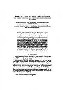
We used SCFT to determine the number of cylindrical phase microdomains that yields the lowest free energy density for a sphere radius of 3 to 4, with χN = 25 and f = 0.8. Initially, several runs were performed starting from random initial conditions, but this approach did not consistently generate the lowest-energy configuration for a given value of R. This is because the SIS algorithm is also capable of relaxing to metastable states [36]. In order to obtain insights into the globally stable solution at each sphere radius, we instead seeded our simulations with density profiles that consist of 10 to 17 cylindrical microdomains for the radii of interest. We believe that these profiles, which were generated from our SCFT simulations starting from random initial conditions and that display the allocation of disclinations observed in the classical Thomson problem [1] for particle-based models, correspond to global minima. In Fig. 1 we present a representative composition profile for the block copolymer cylindrical phase on a sphere—specifically, the case of 12 microdomains covering a sphere. We present more information about the distribution of microdomains that were selected as initial conditions in our SCFT simulations in Appendix C. Using our SCFT model, we determined the number of domains that correspond to the lowest free energy density for a sphere radius between 3 to 4. In Fig. 2 we plot E vs. R for 10 to 17 domains, where the energy density E is approximately equal to the free energy density in the mean-field approximation [36]. From this graph we were able to determine the number of microdomains that correspond to the ground-state configuration for our range of radii. In Fig. 3 we show that as the radius of the sphere is increased, the number of microdomains corresponding to the lowest-energy configuration increases. Of particular interest is the lack of lowest-energy stability regions corresponding to 11 and 13 microdomains. We

8 17 Acquired from SCFT Area Estimate 16

Number of Microdomains

15

14

13

12

11

10

9

8 2.9

3

3.1

3.2

3.3

3.4

3.5

3.6

3.7

3.8

3.9

4

4.1

Sphere Radius, R

FIG. 1: (Color Online). Representative composition profile (bright colors correspond to large A-segment fractions) for the 12 microdomain, ground-state cylindrical phase on the sphere. The key indicates how the coloring corresponds to A-segment fractions. The twelve 5-fold coordinated cylinders are located at the vertices of a regular icosahedron. While the other cylinder phase configurations have a very similar appearance, they have different numbers of microdomains and a different unit cell structure. -0.14 -0.142

Free Energy Density, E

-0.144 -0.146 -0.148 -0.15 -0.152 -0.154 10 Microdomains 11 Microdomains 12 Microdomains 13 Microdomains 14 Microdomains 15 Microdomains 16 Microdomains 17 Microdomains

-0.156 -0.158 -0.16 2.9

3

3.1

3.2

3.3

3.4

3.5

3.6

3.7

3.8

3.9

4

4.1

Sphere Radius, R

FIG. 2: Graph of E vs. R for 10 to 17 microdomains on a sphere. Each data point is the result of a single SCFT simulation seeded with an initial condition with the target number of microdomains. There are regions where 10, 12, 14, 15, and 16 domains are the lowest-energy configuration, while 11 and 13 microdomains are nowhere lowest in energy.

also note that the 12 microdomain configuration, illustrated in Fig. 1, has the lowest energy (is stable) for the largest range of R, while the stability regions corresponding to 10, 14, 15, and 16 microdomains are significantly narrower. Figure 3 also contains an “area estimate” prediction for the number of microdomains covering a sphere. Here, the approximate area for a hexagonal Wigner-Seitz cell (see

FIG. 3: Graph of number of microdomains vs. R for the ground-state (i.e., lowest-energy) configurations. The solid line represents the results obtained through an “area estimate,” while the data points represent data that was acquired from our SCFT simulations. The SCFT simulations indicate that the ground-state configuration contains 10 domains from R = 3 − 3.16, 12 domains from R = 3.17 − 3.73, 14 domains from R = 3.74 − 3.81, 15 domains from R = 3.82 − 3.84, and 16 domains from R = 3.85 − 4.

[21] for a definition of Wigner-Seitz cells) was obtained from a fully relaxed, flat-space unit cell simulation with the same parameters as our block copolymer system. It was determined through this approach, which does not capture the effect of curvature, that a microdomain 6-fold coordinated unit cell occupies an area of approximately 10.6 in flat 2D space. One can divide this approximate Wigner-Seitz cell area into the total surface area 4πR2 of the sphere to obtain an approximation for the number of expected block copolymer microdomains that will cover a sphere of a given radius. There is a striking disagreement between this approximation for the number of microdomains and the observed lowest-energy configurations from the SCFT simulations. The area estimate calculations do not capture the effects of topological constraints, nor the competition between interfacial energy and chain stretching on a curved surface, so we view this deficiency as the primarily reason for the disagreement with SCFT. The cylindrical phase was further studied for larger sphere radii, where we observed structures called grain boundary scars. These results will be presented in Sec. III C.

B.

Cylindrical Phase and the Strong Segregation Limit Approximation

To better understand the behavior observed in the SCFT simulations of cylinder-forming AB diblock copolymers on a sphere, specifically the lack of stable configurations exhibiting 11 or 13 microdomains, we ex-

9

Free Energy Density, ESSL

1.76

1.755

1.75

1.745

10 Microdomains 11 Microdomains 12 Microdomains 13 Microdomains 14 Microdomains 15 Microdomains 16 Microdomains

1.74 4.8

4.9

5

5.1

5.2

5.3

5.4

5.5

5.6

5.7

5.8

5.9

6

Sphere Radius, R

FIG. 4: Graph of ESSL = F/4πR2 vs. R [given by Eq. (C13)] for 10 to 16 microdomains on a sphere. The unit cell configuration used to construct each curve was selected from the observed Wigner-Seitz cell configurations in the SCFT simulations, summarized in Table III. Note the striking qualitative agreement with Fig. 2.

amine a strong segregation limit (SSL) approximation for the free energy F of a thin-film AB diblock copolymer system on a sphere. This calculation is divided into two distinct parts. The first part involves determining the relevant Wigner-Seitz cell configuration for block copolymer microdomains covering a sphere. The second part involves identifying the SSL free energy of each unit cell and summing the SSL free energy over all unit cells on the sphere. We discuss the derivation of the SSL approximation as it applies to the spherical system of interest in Appendix C. In Sec. III B 1 we present the results of the SSL approximation. 1.

SSL Cylindrical Phase Results

In Fig. 4 we plot ESSL = F/4πR2 vs. R for 10 to 16 microdomains on a sphere, were F is the total SSL approximate free energy, Eq. (C13), defined in Appendix C. This figure was constructed using the unit cell configurations from Table III. It is notable that this graph is qualitatively very similar to the E vs. R graph for our SCFT simulations, Fig. 2. Specifically, there is a small region where 10 microdomains is the lowest-energy configuration, there is a large region where 12 microdomains is the lowest-energy configuration, the 13 microdomain configuration is nowhere lowest in energy, there is a large region where 14 microdomains is the lowest-energy configuration, and the 15 microdomain configuration only has a small region of stability. For 13 microdomains, the chain stretching penalty is apparently too great, and both the 12 and 14 microdomain arrangements are lower in energy than the 13 microdomain arrangement over all radii of interest.

In spite of the excellent qualitative agreement, there are a few noticeable differences between Fig. 2 and Fig. 4. First, the scale for R in Fig. 4 is shifted by approximately a factor of 1.5 when compared to Fig. 2. Considering that our system is not strictly in the SSL limit and the spherical SSL free energy involves numerous approximations (specifically, the circular unit cell approximation, the neglect of curvature effects, and the equiareal triangulation—see Appendix C for the descriptions of these approximations), this discrepancy in the scale of R is to be expected. Also, the SSL calculation predicts a small window in R where the 11 microdomain configuration is lowest in energy (specifically, from approximately R = 4.90 − 4.94). The SCFT results do not show the existence of such a region. Again, we believe this disagreement is a consequence of the approximations inherent in the SSL model. Overall, the simple SSL model provides an illuminating picture for how BCP microdomains cover a sphere. Of utmost importance is the effect that topological constraints have on the interfacial and stretching energy of the BCP melt. High-symmetry solutions (e.g., 12 and 14 microdomains) have low-energy unit cell configurations, and low-symmetry solutions (e.g., 11, 13, and 15 microdomains) are characterized by high-energy unit cells.

C.

Grain Boundary Scars in the Cylindrical Phase

As the size of the sphere, and thus the number of microdomains, is increased, isolated 5-fold disclinations become more energetically costly due to the amount of strain they produce. In order to reduce this elastic strain energy, the system introduces dislocations (pairs of 5and 7-fold disclinations). Although some of these dislocations are isolated, a majority of them produce high-angle (30◦ ) curved chains of dislocations called grain boundary scars [6]. These grain boundaries, which have been observed to freely terminate within the lattice, are known to consist of a chain of three to five dislocations, as well as one extra 5-fold disclination; thus, in order to satisfy the required net disclination charge of twelve (c.f., Eq. (2)), there should be a total of twelve grain boundaries on a sphere [6]. These scars, which have been studied both experimentally, on spherical crystals (formed by self-assembled beads on water droplets in oil [6]), and theoretically, through the Thomson problem [13–15], have been observed to appear when the ratio of the sphere radius R to the mean particle spacing d is approximately greater than or equal to five, or when the number of particles exceeds approximately 360 [7]. To determine if our simulations are capable of exhibiting grain boundary scars, a sphere of radius R = 20.0, with f = 0.8 and χN = 25.0, was simulated starting from random initial conditions. The final configuration consisted of 446 microdomains (69 5-fold, 350 6-fold, and 57 7-fold coordinated sites), and, thus, it should exhibit some scaring. To easily visualize these grain boundary

10

FIG. 5: (Color Online). A Voronoi diagram for the cylindrical phase on a sphere of radius R = 20.0, with f = 0.8 and χN = 25.0. The sphere consists of 446 microdomains (69 5fold, 350 6-fold, and 57 7-fold coordinated sites) and exhibits grain boundary scars.

scars, a Voronoi diagram was also produced, and is shown in Fig. 5. Although the sphere does exhibit some scaring, the scars are not arranged symmetrically around the sphere—which is known to be the lowest-energy configuration [6]. This is not surprising since large-cell SCFT simulations started from random initial conditions are well known to produce defective metastable states [36]. The number of metastable states increases rapidly with the total number of domains [12], so SCFT trajectories for large spheres initiated from random initial conditions invariably fail to generate the lowest energy configuration. In the future, we plan to report on the application of annealing techniques to achieve ground state scar structures.

D.

SCFT Lamellar Phase Results

To study the lamellar block copolymer phase on the surface of the sphere, we used SCFT to determine the morphology that yielded the lowest free energy density for a sphere radius of R = 3.1 − 4.9 and R = 10 − 11.8, with χN = 12.5 and f = 0.5. The lamellar block copolymer phase is analogous to the smectic-A phase of liquid crystals [19, 48]. Accordingly, we observe defect structures familiar from liquid crystal theory, and we are compelled to make comparisons of our results with liquid crystal systems. Although the nematic liquid crystal phase constrained to the surface of a sphere has been explored (e.g, see

[24, 25]), studies of smectic ordering in this geometry have been quite limited [22]. The defect configuration with two +1 defects, one on each pole, has been observed (or discussed) in both nematics and smectic-A liquid crystal systems (hedgehog). However, the configuration with four + 12 defects differs between the two systems. For a nematic, the + 21 defects are located on the vertices of a tetrahedron (baseball) [24, 25], while for a smectic-A they all lie on a great circle, each separated by 90◦ (quasi-baseball) [22]. This is due to the different elastic properties of the two systems. A discussion of +1 and + 12 defect structures in liquid crystals can be found in de Gennes and Prost [19]. In Fig. 6 we summarize the defect structures that were observed in our SCFT simulations of lamellar block copolymers on a sphere. We observed both the hedgehog and quasi-baseball defect structures as described above. However, we also observed a variant of the quasi-baseball where the four + 21 defects are located on a great circle, but are not separated by 90◦ (spiral). This defect state resembles a double spiral. All three of these configurations were also recently identified by Li et al. [32]. The presence of these three defect configurations in our SCFT simulations is not surprising. In fact, related states can be systematically constructed from the simple hedgehog state. If we cut the hedgehog sphere perfectly along a great circle that intersects the two +1 defects, and then rotate one of the hemispheres by an integer number of lamellar spacings, we can construct a wide range of quasi-baseball and spiral defect structures. Clearly, transitions between the various lamellar defect configurations will not proceed by such a transformation, but this cut-and-rotate exercise is useful for visualizing the defect structures. In our SCFT simulations, we observed an R-dependent transition in lowest-energy configuration from a smecticA texture with two singular +1 defects (hedgehog) to a configuration with four + 21 defects (spiral) and vice versa. To facilitate a quantitative study of the energetics of competing structures, three configurations were seeded into our simulations, the quasi-baseball, hedgehog, and spiral structure, in the same manner as was done for the cylindrical phase. Although the spiral and quasi-baseball structure both have four + 12 defects, they differ in the number of continuous lamellae stripes they contain on their surface, and in the positioning of those stripes. The spiral structure contains one continuous lamellar stripe, while the quasi-baseball structure contains two or more stripes. Furthermore, on the quasi-baseball, the defects are equally spaced at 90◦ intervals on a great circle, while on the spiral, the four defects are not necessarily evenly spaced. In Figs. 7 and 8, we show the free energy density versus sphere radius determined from SCFT simulations of the competing hedgehog, quasi-baseball, and spiral phases. These studies, which were conducted with parameters χN = 12.5 and f = 0.5, identify the ground state configuration for two intervals of sphere radii: R = 3.1 − 4.9

11

FIG. 6: (Color Online). Three lamellar configurations (density composition profiles where bright colors correspond to large A-segment fractions) that were obtained and studied through our SCFT simulations. Again, the key indicates how the coloring corresponds to A-segment densities. (a), (d), and (g) are flat 2D projections of the spiral, hedgehog, and quasibaseball phases, respectively. (b), (e), and (h) are the spiral, hedgehog, and quasi-baseball phases, respectively, projected on the surface of a sphere. (c), (f), and (i) are slices of the 2D spherical projections, which show that the defects of these lamellae phases all lie on a great circle.

and R = 10 − 11.8. For the interval R = 3.1 − 4.9, the hedgehog is consistently the lowest-energy configuration, except at R = 3.88. For the interval R = 10 − 11.8, we observe an alternation in stability between the hedgehog and the spiral defect structures. E.

Analogy with Smectic-A Liquid Crystals 1.

2.

Applicability of Smectic-A Models

As discussed in de Gennes and Prost [19], the elastic energy density (per unit area) of the smectic-A phase can be approximated in flat space as: fsmA =

1¯ 2 1 Bǫ + K1 σ 2 , 2 2

transition. For block copolymers, λ ≈ 0.1d, where d is the lamellar repeat spacing [48, 49]. For a confined smectic-A system, we expect a competition between the bending and compression degrees of freedom that is dependent on the confinement scale. Indeed, commensurability is less of a factor for large confinements. The characteristic confinement length of a smectic-A system L sets the order of magnitude of the lamellar bending [22]. For a large confinement λ ≪ L, and compression effects are negligible: ǫ ≪ λ/R and ¯ 2 ≪ K1 σ 2 [22]. Bǫ For the spherical system of interest here, the natural confinement length is set by the sphere radius R. Therefore, we expect layer compression, and consequently lamellar commensurability, to play less of a role in selecting lowest-energy configurations for large sphere radii. Furthermore, it is reasonable to assume that commensurability effects play a more important role in selecting lowest-energy configurations for small sphere radii. It is interesting to note that for R = 3.1 − 4.9 the sphere radius is comparable to the lamellar spacing, d. Elastic liquid crystal theories have a short-length-scale cutoff, below which elastic theory does not apply. This cutoff often corresponds to the liquid crystal defect core radius, which, for a smectic-A liquid crystal, is of order the layer repeat spacing. Therefore, our spherical BCP lamellar system lies outside the applicable range of classic liquid crystal theory for small sphere radii. For the interval R = 10 − 11.8, the sphere radius is still relatively small, but likely inside the applicable range of elastic liquid crystal theory. Therefore, according to the above argument, we expect the dilation-compression mode to play an important role in determining the lowestenergy state. With this in mind, the observed alternation between hedgehog and spiral defects in Fig. 8 is not surprising. For even larger sphere radii, perhaps of order R = 100, we expect dilation-compression effects to have less of a direct effect and the alternation between ground states to be less pronounced (and perhaps non-existent).

(46)

¯ and K1 are the dilation (compression) modulus where B and mean curvature (bending) modulus, respectively, ǫ is a strain of dilation (compression), and σ is a bending strain. The ratio of the two moduli is often expressed as ¯ where λ is a length scale that is comparable λ2 = K1 /B, to the layer thickness when the system is far from a phase

Quasi-Baseball/Spiral Defect Configurations as a Helfrich-Hurault Transition

In order to understand the mechanism driving the hedgehog–quasi-baseball/spiral transitions for large sphere radii, we can examine Eq. (46) and an approximate analytic result. Comparing the two defect structures, we can see that the hedgehog morphology exhibits minimal dilation (here we use the term “dilation” to refer to dilation or compression, as they represent the same degree of freedom) when the sphere circumference is an integer multiple of the lamellar spacing, while dilation can be large for intermediate values of sphere circumference (i.e., not corresponding to an integer number of lamellar spacings). To compensate for the high dilation at intermediate values of sphere radius, the quasi-baseball/spiral

12 -0.8 Quasi-Baseball Hedgehog Spiral

TABLE I: Values of Rhn and Rsn obtained from Eqs. (47) and (48), respectively. Only values of R in the interval of our SCFT simulations (R = 3.1 − 4.9 and R = 10 − 11.8) are reported. Table II provides similar data collected from the SCFT simulations.


-0.82

-0.84

-0.86

n 6 7 8 18 19 20 21

-0.88

-0.9

-0.92

Rhn 3.32 3.87 4.43 10.52 11.07 11.63

Rsn 3.60 4.15 4.71 10.25 10.80 11.35 -

-0.94 3

3.2

3.4

3.6

3.8

4

4.2

4.4

4.6

4.8

5

Sphere Radius, R

FIG. 7: E vs. R for the lamellar phase on a sphere from SCFT simulations for f = 0.5 and χN = 12.5. For the radius range of R = 3.1 − 4.9, the hedgehog structure was the observed lowest-energy configuration except at R = 3.88. -0.966 Quasi-Baseball Hedgehog Spiral

-0.968


-0.97 -0.972

TABLE II: Values of Rh and Rs obtained from the approximate minima of the hedgehog and spiral E vs. R curves, respectively, in Figs. 7 and 8. Rh 3.62 4.20 4.78 10.30 11.40

Rs 10.90 -

-0.974 -0.976 -0.978 -0.98 -0.982 -0.984 -0.986 9.8

10

10.2

10.4

10.6

10.8

11

11.2

11.4

11.6

11.8

12

Sphere Radius, R

FIG. 8: E vs. R for the lamellar phase on a sphere from SCFT simulations for f = 0.5 and χN = 12.5. For the interval R = 10−11.8 the hedgehog (R = 10−10.54 and R = 11.08−11.77) and spiral (R = 10.6 − 11.05 and R = 11.8) configurations alternate as the ground state.

arrangement produces areas of curvature (bend) that, in turn, relieve dilation, and thus lower the overall free energy. To determine the approximate radii Rhn where the hedgehog structure is lowest in energy, we assume that the circumference of the sphere is equal to an integer number of lamellar periods nd: Rhn =

nd . 2π

(47)

When the radius of the sphere is increased or decreased from these optimum values for the hedgehog morphology, there is a large elastic energy contribution from lamellar compression or dilation, and a Helfrich-Hurault transition occurs, where the lamellar layers exhibit undulations

to fill the extra space produced by expanding the system [19]. We believe that the spiral (and quasi-baseball) structures are obtained through this type of transition, where layer bending substitutes for layer compression or dilation. The radius Rsn where the spiral (or perhaps the quasi-baseball) morphology is lowest in energy can be roughly approximated by: n + 12 d Rsn = , (48) 2π where the extra term of + 21 represents the intermediate sphere radii where the circumference is not a full integer multiple of the lamellar repeat spacing. From this simple calculation, we expect that there will be alternating regions where one defect morphology will be lower in energy than the others. To calculate the natural lamellae repeat spacing d, a fully relaxed unit cell calculation in flat space was performed using the same system parameters (i.e., f = 0.5 and χN = 12.5). From this simulation we found that d ≈ 3.48. Using Eqs. (47) and (48), we can calculate the approximate radii where the hedgehog structure and spiral (or quasi-baseball) structure are predicted to be lowest in energy. These results are summarized in Table I. Note that the results in Table I approximately agree (at least qualitatively) with the behavior observed in our SCFT simulations for large R, summarized in Fig. 8 and Table II. At small sphere radii, the above commensurability calculation fails to provide a qualitative explanation for the

13 SCFT results, although it does roughly correlate with the near-stability of the spiral phase at R ≈ 3.3, 3.9, and 4.4. At larger radii, 10 < R < 12, the commensurability argument becomes semi-quantitative and alternating regions of spiral and hedgehog stability are observed. For even larger spheres, we expect that the energetics of dilationcompression of the layers will be less important and that the ground state morphology will be dictated to a larger extent by layer bending forces.

3.

Quasi-Baseball and Spiral Defect Configurations

As mentioned above, the topological defect structure of the quasi-baseball and the spiral configurations are very similar. The primary difference is the observed location of the + 21 defects. For large R, we argued that the spiral configuration relieves elastic compression-dilation frustration by introducing layer bending. However, the quasi-baseball structure is an alternate structure that substitutes lamellae bending for layer compressiondilation. One possible explanation for the observed stability of spiral relative to baseball structures in our SCFT simulations is that for a given sphere radius, there are only two possible quasi-baseball structures, whereas the spiral has many different manifestations. For example, the + 21 defects on the spiral can be separated by 1 or more lamellae stripes and the spiral can have varying degrees of “twist.” Accordingly, it is reasonable to expect that the more “compliant” spiral structure will have a lower energy than the quasi-baseball structure over a broader range of sphere radii.

F.

The Role of Fluctuations

By using the mean-field (SCFT) approximation to simplify our field-theoretic model, we ignore field fluctuations that are otherwise present in the model and can play a role in experimental systems. In flat-space, two-dimensional systems and bulk block copolymers in three-dimensions, field fluctuations can have the effect of shifting phase boundaries and stabilizing the disordered phase relative to the ordered microphases [36]. In the context of the present work, fluctuations could be especially important in determining the relative stability of phases on the sphere when the mean-field free energy densities of competing phases are close in magnitude (see Figs. 2, 7, and 8). We expect that lower symmetry phases, e.g. spirals and baseballs, which possess easily excitable undulation modes on the sphere, will be fluctuation-stabilized relative to higher symmetry phases in such circumstances. In any event, the importance of fluctuations can be controlled by the Ginzburg parameter C and strictly eliminated in the limit C → ∞ where mean-field theory becomes exact. Experimentally this can be approached by working with copolymer melts of very high molecular weight. Fluctuation effects could

also be theoretically explored in the present model by conducting stochastic complex Langevin simulations [36], although such simulations would be considerably more expensive than the SCFT calculations reported here.

IV.

CONCLUSIONS

We presented a new spectral collocation scheme for developing numerical SCFT solutions of inhomogeneous polymers confined to the surface of a sphere. We believe that our numerical methods are the most accurate and efficient available for the spherical geometry and represent a significant advance over previous finite difference and finite volume approaches. In application to a standard model of AB diblock copolymer melts confined to a thin film on a sphere, we used numerical SCFT to study defect structures that arise due to a spherical geometry. Specifically, we determined ground-state configurations for both the lamellar (χN = 12.5, f = 0.5) and cylindrical (χN = 25, f = 0.8) phases. For the cylindrical phase, we found that there was a delicate competition between topological constraints and chain stretching that selected the ground-state microdomain configuration observed on the sphere. In the SCFT simulations, configurations with 11 and 13 cylindrical microdomains were never observed to be lowest in energy. We believe that the topological constraints for such configurations resulted in unit cell structures that contained excessive amounts of chain stretching, and thus a high free energy relative to other microdomain configurations. Although our model was also capable of producing grain boundary scars for large sphere simulations of the cylindrical phase, additional work will be required to investigate the ground-state configuration. Because of the large sphere size required to obtain scar structures and the high spatial resolution required for accurate free energy evaluation, it is computationally difficult to apply SCFT in this context. For the lamellar phase, we found that for small sphere radii, the hedgehog defect configuration was almost always lowest in energy. For larger sphere radii there was competition between the hedgehog and spiral defect configurations. Quasi-baseball configurations, with defect structures closely related to the spiral, were found to be metastable, but close in energy to the spiral, especially in regions of sphere radius where the hedgehog was strongly disfavored. To qualitatively explain the SCFT results, analytic approximations using microdomain packing arguments, elastic liquid crystal models, and the BCP strong segregation limit were also presented. While not as robust as SCFT, these calculations provided useful insights into the driving forces behind the observed BCP microdomain and defect structures on the surface of a sphere. In this study, we considered a diblock copolymer thin film on the surface of a sphere, where the system is uni-

14 form but thin in the radial direction. These conditions may be difficult to realize experimentally, such as in colloids and nanoparticles coated with a thin layer of block copolymer. Specifically, it might prove difficult to neutralize both inner and outer surfaces of the layer, so that the block copolymer microphases “stand up” and are compositionally homogeneous in the radial coordinate. The thinness constraint is less problematic, because as the radius of the sphere is increased into the colloidal domain, it becomes more experimentally viable to produce thin films satisfying the inequality R ≫ h. For a more detailed investigation of the ground state configuration on small spheres, or under conditions where preferential wetting occurs on the inner or outer surfaces of the copolymer film, it may be necessary to abandon our 2D model and invest in a full 3D SCFT calculation. We plan to conduct future studies along these lines that will enable the design of functional colloids and nanoparticles with copolymers adsorbed, coated, or grafted on their surfaces.

c V. 2

E=

(A2)

Therefore, Eq. (A1) becomes χE = F +

2−c V. 2

(A3)

Let Nz be the number of polygons in the covering with exactly z sides. Then, X F = Nz , (A4) z

and X

zNz = cV.

(A5)

z

This last formula follows because each vertex is common to exactly c polygons. ¿From Eqs. (A3), (A4), and (A5), it follows that X 2c 2c X 2c χE = F +cV = Nz + zNz , (A6) 2−c 2−c 2−c z z

Acknowledgments

The authors would like to thank Kirill Katsov, Richard Elliot, David R. Nelson and Vincenzo Vitelli for insightful discussions. We also wish to thank Erin Lennon for providing the flat-space, unit cell SCFT results used to determine lattice constants for the cylindrical and lamellar phases. TLC received partial funding through NSF IGERT grant DGE02-21715. GHF, CJGC, TLC, and AWB derived partial support from NSF grant DMR0603710 and the MARCO Center on Functional Engineered Nano Architectonics (FENA), while EJK and AH derived partial support from NSF grant DMR-0307233. AWB received additional support from The Frank H. and Eva B. Buck Foundation. The work of CJGC was funded by NSF grant DMS-0505738. HDC acknowledges partial support from NSF grant DMS-0609996. This work made use of MRL Central Facilities supported by the MRSEC Program of the National Science Foundation under Award No. DMR05-20415.

APPENDIX A: DERIVATION OF EQ. (2) FROM ´ FORMULA THE EULER-POINCARE

Consider a compact manifold M without boundary with Euler-Poincaré characteristic χE . Further consider a covering of M by polygons. The Euler-Poincaré characteristic of M is defined as χE = F − E + V,

each vertex, then we find:

(A1)

where F , E, and V are the number of faces, edges, and vertices in the covering, respectively. If we restrict our attention to coverings where exactly c edges intersect at

which can be simplified to obtain X 2c 2c − z Nz = χE . c − 2 c −2 z

(A7)

With the assumption that exactly three edges intersect at each vertex, c = 3 and Eq. (A7) can be rewritten as: 1X (6 − z)Nz = χE , 6 z

(A8)

which is identical to Eq. (2). APPENDIX B: SPHEREPACK 3.1 AND NUMERICAL METHODS

Although there are several choices of basis functions that can be used for spectral collocation solutions on the sphere, spherical harmonics are the most “ideal” due to their properties of completeness, orthogonality, exponential convergence (for functions that are infinitely differentiable on the sphere), and equiareal resolution. The spherical harmonic basis also circumvents the “pole problem,” which is often encountered in algorithms that utilize a finite difference or finite element grid. Thus, with spherical harmonics, features on the sphere are equally resolved independent of the location of the poles. More information about the spherical harmonics basis and the pole problem can be found in [40, 50, 51]. As mentioned above, spherical harmonics are also desirable because they are the eigenfunctions of the twodimensional Laplacian operator in spherical coordinates ∇2u Ylm (u) = −l(l + 1)Ylm (u).

(B1)

15 This property, which closely mimics the Fourier basis in flat Euclidian space with periodic boundary conditions, makes it possible to efficently calculate the Laplacian in the modified diffusion equations [e.g., Eq. (12)] through the method explained in Sec. II C. In order to simulate the block copolymer system of interest it is necessary to discretize the variables φ and θ. It proves convenient to utilize a 2D equally spaced grid in colatitude and longitude to discretize our system. Specifically, we define: θi = Nπi −1 , i = 0, ..., N − 1 φj = 2πj M , j = 0, ..., M − 1

(B2)

where N and M are the total number of grid points in the θ and φ directions respectively. We will use the symbol i to refer to the ordered pair (i, j). The chain contour variable s and the fictitious time variable t are also sampled on discrete intervals: sµ = nµs , µ = 0, ..., ns tn = n∆t, n = 0, ..., nt

(B3)

where ns and nt are the number of contour steps on the polymer backbone and the number of iterations that are utilized to relax the SCFT equations, respectively. The choice of SCFT time step ∆t depends on the method used to integrate Eqs. (27) and (28). In order to easily transform between real and lmspace, we use a package of FORTRAN 77 subroutines, SPHEREPACK 3.1, which were produced by John Adams and Paul N. Swarztrauber of the National Center for Atomospheric Research [40]. Since our SCFT equations only involve real-valued scalar functions, the real representation of the transforms that this software library utilizes is ideal because it requires only half the computation associated with the complex form represented in Eq. (31) [52]. The subroutines use the following “triangular truncated” expression for the spherical harmonic expansion, which allows us to approximate a smooth function f (u) to arbitary precision for some integer value of L [40]: f (u) ≈

L X l X

Plm (θ)(alm cos(mφ) +

l=0 m=0

blm sin(mφ)).

grid, SPHEREPACK 3.1 utilizes the method of Machenhauer and Daley [40], which is known to have the same high level of accuracy as Gaussian quadrature. More details about the actual method can be found in Ref. [53]. The main computational difficulty associated with the spherical harmonic basis is the lack of a fast Legendre transform. Since the basis is a Fourier series in longitude, FFT algorithms can be used to efficently calculate the Fourier transforms in this one dimension. Significantly more computational time is spent performing the Legendre transform in colatitude. The overall operation count for a transform or inverse transform utilizing a triangular truncation with L2 spherical harmonics is O(L3 log2 L) operations [50]. APPENDIX C: DERIVATION OF THE SSL FREE ENERGY FOR THE CYLINDRICAL PHASE IN A SPHERICAL THIN FILM a.

Approximate SSL Free Energy for the Cylindrical Phase

We begin with an approximate free energy of a WignerSeitz cell valid in the strong segregation limit (i.e., χN ≫ 10) [54, 55]: Fc = Fcore + Fcorona + Finterface .

(C1)

where Fcore is the chain-stretching free energy of the cylindrical core of the circular unit cell, Fcorona is the chain-stretching free energy of the corona of the circular unit cell, and Finterface is the interfacial energy of the core-corona interface (i.e., the B-A interface). The circular Wigner-Seitz cell approximation is utilized by replacing the actual Wigner-Seitz corona boundary by a circle of radius Rc . The radius Rc is selected by requiring that the circular unit cell have the same total area as the actual Wigner-Seitz cell. The details of this model can be found in the literature (c.f., [54, 55]). Here we are primarily concerned with the functional form of each term. Specifically, from Ref. [55], π 2 πhb2 Fcore = Rc4 , (C2) 96 6ν0

(B4)

Since spherical harmonics are a Fourier series in longitude, the longitudinal grid points are most optimal when they are evenly spaced, but this is not the case in the colatitude direction since a simple FFT cannot be used [50]. There are currently several methods that can be applied to calculate these transforms using either an equally spaced or Gaussian grid in colatitude [51], and in order to account for this choice there are two versions of each SPHEREPACK 3.1 subroutine. The calculations reported in this paper were performed using the version that applies an evenly spaced grid in both coordinates, as described above. For the uniform colatitude

Fcorona =

πhb2 1 1 Rc4 , log 16 (1 − f ) 6ν0

(C3)

and Finterface

p = 2 6(1 − f )χN

πhb2 6ν0

Rc ,

(C4)

where Rc is in units of the unperturbed radius of gyration Rg0 . As before, h is the thickness of the BCP thin film, b is the statistical segment length, ν0 = 1/ρ0 is the average segment volume, N is the total number of segments per chain, f is the fraction of A segments (we have assumed

16 that f > 0.5), and χ is the A-B Flory interaction parameter. Combining terms, we find that the free energy in Eq. (C1) can be expressed in the more compact form πhb2 πhb2 Fc = CI Rc + CS Rc4 , (C5) 6ν0 6ν0

TABLE III: Relevant Wigner-Seitz cells for M = 10, 11, .., 16 microdomains on a sphere. This table reflects only a small fraction of the geometrically allowed unit cells; however, these unit cell configurations are consistent with ground-state SCFT configurations of BCP on a sphere and with groundstate configurations of the Thomson problem [1].

where the first term captures the energy associated with interfacial tension, the second term captures the energy associated with chain stretching, and CI and CS are f and χN -dependent parameters. Dividing both sides of Eq. (C5) by πhb2 /6ν0 yields a dimensionless free energy F˜c ,

M 10 11 12 13 14 15 16

F˜c = CI Rc + CS Rc4 ,

and

π2 1 1 CS = , + log 96 16 1−f

(C7)

(C8)

For the system of interest here, with f = 0.8 and χN = 25, CI ≈ 10.9545 and CS ≈ 0.2034. We need to determine the area of the Wigner-Seitz cell so that we can calculate the corresponding circular unit cell radius Rc . Provided we know the type, number, and area of all microdomain unit cells covering a sphere, we can generate an approximate free energy of the block copolymer thin-film by summing up the SSL free energies for all unit cells. This approximation does not explicitly address curvature. Furthermore, our simulations with χN = 25 are not strictly in the strong segregation limit [56]. However, we believe that the primary forces driving the observed spherical microdomain unit cell structures are a combination of stretching energy, interfacial energy, and geometric packing (enforced by topological constraints). This rudimentary SSL model, coupled with some simple geometric arguments, can capture all three of these elements. b.

N5 8 8 12 10 12 12 12

N6 0 1 0 2 2 3 4

(C6)

where p CI = 2 6(1 − f )χN,

N4 2 2 0 1 0 0 0

Wigner-Seitz Cells and SSL Free Energy on a Sphere

In order to apply the SSL free energy discussed above, we need to determine the relevant Wigner-Seitz cell configurations on the sphere. Furthermore, if we are interested in the dependence of SSL free energy on the sphere radius R, then we need to determine how the unit cell areas depend on R. This will allow us to connect the circular unit cell radius Rc to the sphere radius R. Let SR represent a sphere of radius R and M represent the total number of minority (B-block) microdomains covering SR . Figure 1 illustrates the example of 12 B domains covering a sphere. For a specific microdomain on

SR , the number of nearest-neighbor B domains is given by the number of sides of the microdomain’s WignerSeitz cell. The total number of z-gon Wigner-Seitz cells on SR is denoted Nz (equivalently, this is the number of z-fold coordinated microdomains). A specific unit cell configuration of M microdomains on SP R is given by the set of all Nz ; we denote this set {Nz | z Nz = M }, or {Nz }M for short. Note that the set {Nz }M is not unique. However, for non-degenerate ground-states, only one set {Nz }M is physically relevant (for small M , we expect the lowest-energy configuration is non-degenerate), but from a purely geometric and topological standpoint, many different unit cell configurations are possible. Perhaps the easiest way to identify the physically relevant {Nz }M is to perform a Voronoi analysis on the density composition profiles output by our SCFT simulations, as a Voronoi analysis provides the Wigner-Seitz cell structure (see [57] for details about Voronoi analysis of BCP density profiles). For the cases of M = 10, 11, ..., 16, Table III summarizes the observed WignerSeitz cell structure obtained from Voronoi analysis of the SCFT density profiles. These are the same configurations used to seed the simulation results presented in Sec. III A. We note that the observed distribution of Voronoi cells for M microdomains on a sphere is consistent with the known results of the M -particle Thomson problem (i.e., the problem of finding the ground state of M particles constrained to a sphere, interacting via the Coulomb potential [1]). We still need to calculate the unit cell areas in order to apply Eq. (C6) to sum the SSL free energy over the sphere. All relevant unit cell polygons (i.e., square, pentagon, and hexagon) can be constructed from triangles: a square is made up of 4 triangles, a pentagon is made up of 5 triangles, and a hexagon is made up of 6 triangles. For a regular n-gon, the area of the polygon is given by An = nATn , where ATn is the area of each triangle. Figure 9 provides a schematic of the relevant unit cells, and the appropriate decomposition into component triangles. In general, the unit cells will not always be regular polygons, and the triangles will not all have the same area; in general, ATn 6= ATm , for n 6= m. However, if we make

17 2. We assume the area of an z-gon Wigner-Seitz cell is given by Az = zAT . Note that AT , and thus Az , is a function of the sphere radius R.

FIG. 9: Schematics of (a) approximate circular, (b) square, (c) pentagon, and (d) hexagon Wigner-Seitz cells. Note that for each of the polygon unit cells, the component triangles have been drawn. Our approximation assumes that the area of all triangles, in all unit cells covering the sphere, is given by AT [see Eq. (C10)]; thus, the area of an n-gon unit cell is approximated by An = nAT . The radius of the approximate circular unit cell Rc is determined by requiring that circular unit cell area πRc2 is equal to the area of the actual WignerSeitz cell, or in our case, the approximate n-gon unit cell area, An .

two approximations, we can simplify the calculation significantly. When calculating the approximate areas of the Wigner-Seitz cells, we make two assumptions: 1. We assume that the sphere is covered with an equiareal, triangular array, where the total number of triangles nT is calculated using {Nz }M as follows: X nT = zNz . (C9)

While this method only yields approximate unit cell areas, it is reasonably consistent with published results relating the relative sizes of BCP Wigner-Seitz cells. From above, we see that A5 /A6 = 5/6 ≈ 0.83 and A7 /A6 = 7/6 ≈ 1.17. Hammond et al. report that A5 /A6 is between 0.80 and 0.90, and A7 /A6 is between 1.13 and 1.20, depending on the method used to calculate the unit cell area [58]. We note that while the SSL unit cell energies are evaluated in flat space, the equiareal, equilateral triangulation does account for the topological constraints of the sphere. We are now in a position to calculate an approximate SSL free energy of a thin film of microphase separated cylinders covering a sphere of radius R. For a given configuration {Nz }M , we can use the above two assumptions to calculate the areas of all Wigner-Seitz cells on the sphere. This, in turn, allows us to estimate the SSL free energy. This procedure is outlined as follows: 1. Given the Wigner-Seitz cell structure {Nz }M on SR , calculate nT using Eq. (C9) and AT by means of Eq. (C10). 2. For all relevant coordination numbers z, calculate the circular Wigner-Seitz cell radius Rcz : Rcz =

r

zAT . π

(C11)

This gives the radius of the circular Wigner-Seitz cell in terms of the sphere radius. 3. For all relevant coordination numbers z, calculate the SSL approximate free energy F˜cz : F˜cz (R) = F˜c (Rcz ) .

(C12)

z

The area of each triangle is given by AT =

4πR2 . nT

(C10)

Recent work by Travesset [12] suggests that the general problem of finding the lowest-energy state for a collection of constrained particles (in this case, topologically constrained) is equivalent to finding the particle distribution which is nearest to a perfect, equilateral triangulation. Accordingly, our approximate triangulation seems reasonable.

4. The total SSL approximate free energy over the sphere is given by: F (R, {Nz }M ) =

X

Nz F˜cz (R).

(C13)

z

For the purpose of comparing to the SCFT simulations results, we elect to plot the free energy density ESSL ≡ F/4πR2 in Fig. 4. In Sec. III B 1 we used Eq. (C13) to evaluate the SSL free energy for the unit cell configurations summarized in Table III.

18

[1] J. J. Thomson, Philosophical Magazine 7, 237 (1904). [2] B. K. Ganser, S. Li, V. Y. Klishko, J. T. Finch, and W. I. Sundquist, Science 283, 80 (1999). [3] C. Varea, J. L. Aragon, and R. A. Barrio, Physical Review E 60, 4588 (1999). [4] J. Heuser, Journal of Cell Biology 108, 401 (1989). [5] G. G. T. Kohyama, D. M. Kroll, Physical Review E 68, 061905 (2003). [6] A. R. Bausch, M. J. Bowick, A. Cacciuto, A. D. Dinsmore, M. F. Hsu, D. R. Nelson, M. G. Nikolaides, A. Travesset, and D. A. Weitz, Science 299, 1716 (2003). [7] T. Einert, P. Lipowsky, J. Schilling, M. J. Bowick, and A. R. Bausch, Langmuir 21, 12076 (2005). [8] P. Leiderer, Zeitschrift f¨ ur Physik B 98, 303 (1995). [9] M. J. Bowick, D. R. Nelson, and A. Travesset, Physical Review B 62, 8738 (2000). [10] A. Travesset, Physical Review B 68, 115421 (2003). [11] S. Schneider and G. Gompper, Europhysics Letters 70, 136 (2005). [12] A. Travesset, Physical Review E 72, 036110 (2005). [13] M. J. Bowick, A. Cacciuto, D. R. Nelson, and A. Travesset, Physical Review Letters 89, 185502 (2002). [14] M. J. Bowick, A. Cacciuto, D. R. Nelson, and A. Travesset, Physical Review Letters 89, 249902 (2002). [15] M. J. Bowick, A. Cacciuto, D. R. Nelson, and A. Travesset, Physical Review B 73, 024115 (2006). [16] D. R. Nelson, Physical Review Letters 50, 982 (1983). [17] J. P. Gaspard, J. F. Sadoc, and R. Mosseri, in 2nd International Conference on The Structure of Non-Crystalline Materials, Cambridge 1982 (Taylor and Francis, London, 1982). [18] S. Sachdev and D. R. Nelson, Journal of Physics C 17, 5473 (1984). [19] P. G. de Gennes and J. Prost, The Physics of Liquid Crystals (Oxford Science Publications, New York, 1993). [20] F. C. Frank, Dissussions of the Faraday Society 25, 19 (1958). [21] P. M. Chaikin and T. C. Lubensky, Principles of condensed matter physics (Cambridge University Press, Cambridge, 1995). [22] C. Blanc and M. Kleman, The European Physical Journal E 4, 241 (2001). [23] R. D. Kamien, Reviews of Modern Physics p. 953 (2002). [24] D. R. Nelson, Nano Letters 2, 1125 (2002). [25] T. C. Lubensky and J. Prost, J. Phys. II France 2, 371 (1992). [26] W. Helfrich, Zeitschrift f¨ ur Naturforschung C 28, 693 (1973). [27] A. E. Lobkovsky and T. A. Witten, Physical Review E 55, 1577 (1997). [28] V. Vitelli and A. M. Turner, Physical Review Letters 93, 215301 (2004). [29] V. Vitelli and D. R. Nelson, Physical Review E 70, 051105 (2004). [30] V. Vitelli, Ph.D. thesis, Harvard (2006). [31] P. Tang, F. Qiu, H. Zhang, and Y. Yang, Physical Review E 72, 016710 (2005). [32] J. F. Li, J. Fan, H. D. Zhang, F. Qiu, P. Tang, and Y. L. Yang, The European Physical Journal E 20, 449 (2006).

[33] J.-R. Roan, Physical Review Letters 96, 248301 (2006). [34] E. Helfand, Journal of Chemical Physics 62, 999 (1975). [35] M. W. Matsen and M. Schick, Physical Review Letters 72, 2660 (1994). [36] G. H. Fredrickson, The Equilibrium Theory of Inhomogenous Polymers (Clarendon Press, Oxford, 2006). [37] M. W. Matsen, Journal of Chemical Physics 106, 7781 (1997). [38] M. W. Matsen, Current Opinion in Colloid & Interface Science 3, 40 (1998). [39] D. Gottlieb and S. A. Orszag, Numerical Analysis of Spectral Methods: Theory and Applications (Society for Industrial and Applied Mathematics (SIAM), Philadelphia, 1977). [40] J. Adams and P. N. Swarztrauber, Spherepack 3.1: A model development facility (2003), URL http://www. scd.ucar.edu/css/software/spherepack. [41] K. O. Rasmussen and G. Kalosakas, Journal of Polymer Science Part B: Polymer Physics 40, 1777 (2002). [42] F. S. Bates and G. H. Fredrickson, Annual Review of Physical Chemistry 42, 525 (1990). [43] G. H. Fredrickson, V. Ganesan, and F. Drolet, Macromolecules 35, 16 (2002). [44] J. J. Sakurai, Modern Quantum Mechanics, Revised Edition (Addison Wesley, Reading, MA, 1994). [45] M. Frigo and S. G. Johnson, Proceedings of the IEEE 93, 216 (2005). [46] G. B. Arfken and H. J. Weber, Mathematical Methods for Physicists (Academic Press, San Diego, 1995), 4th ed. [47] H. D. Ceniceros and G. H. Fredrickson, Multiscale Modeling & Simulation p. 452 (2004). [48] K. Amundson and E. Helfand, Macromolecules 26, 1324 (1993). [49] C. Harrison, Z. Cheng, S. Sethuraman, D. A. Huse, P. M. Chaikin, D. A. Vega, J. M. Sebastian, R. A. Register, and D. H. Adamson, Physical Review E 66, 011706 (2002). [50] J. P. Boyd, Chebyshev and Fourier Spectral Methods (Dover, Mineola, New York, 2000). [51] P. N. Swarztrauber, SIAM Journal on Numerical Analysis 16, 934 (1979). [52] P. N. Swarztrauber, Monthly Weather Review 121, 3415 (1993). [53] B. Machenhauer and R. Daley, A baroclinic primitive equation model with spectral representation in three dimensions (1972). [54] A. N. Semenov, Soviet Physics JETP 61, 733 (1985). [55] G. H. Fredrickson, Macromolecules 26, 4351 (1993). [56] Numerical SCFT is difficult at χN ≫ 25 because the interfacial scale becomes much narrower than the microdomain period and a large amount of spatial and contour resolution is required [59]. [57] R. A. Segalman, A. Hexemer, R. C. Hayward, and E. J. Kramer, Macromolecules 36, 3272 (2003). [58] M. R. Hammond, S. W. Sides, G. H. Fredrickson, E. J. Kramer, J. Ruokolainen, and S. F. Hahn, Macromolecules 36, 8712 (2003). [59] M. W. Matsen, Journal of Chemical Physics 114, 10528 (2001).

Self-consistent field theory simulations of block ... - Semantic Scholar

Self-consistent field theory simulations of block ... - Semantic Scholar

Suggest Documents

Selfconsistent theory of block copolymer blends

SelfConsistent Field Theory for the Electronic

Selfconsistent modeling of the largescale ... - Semantic Scholar

Quantum Field Theory - Semantic Scholar

An inhomogeneous selfconsistent reaction field ...

Lattice field theory simulations of Dirac semimetals

Field Measurements and Numerical Simulations of ... - Semantic Scholar

Phase-field simulations of velocity selection in ... - Semantic Scholar

scaling theory and computer simulations of termite ... - Semantic Scholar

A selfconsistent fully turbulent theory of auroral ... - Wiley Online Library

Theory of chemical exchange in zero field NMR - Semantic Scholar

Covariant Field Theory on Frame Bundles of ... - Semantic Scholar

The Electromagnetic Field Theory of Consciousness - Semantic Scholar

A dynamical theory of the electromagnetic field - Semantic Scholar

Quantum field theory of photons with orbital ... - Semantic Scholar

Polymer Field-Theory Simulations on Graphics Processing Units

Non-linear Osmotic Brush Regime: Simulations and mean-field theory

Managing access block - Semantic Scholar

Suprascapular nerve block - Semantic Scholar

BLOCK STRUCTURED QUADRATIC ... - Semantic Scholar

Loose graph simulations - Semantic Scholar

computer simulations and theory

EVALUATION OF WAVELET DOMAIN BLOCK ... - Semantic Scholar

EVALUATION OF WAVELET DOMAIN BLOCK ... - Semantic Scholar