Semantic Image Based Geolocation Given a Map
arXiv:1609.00278v1 [cs.CV] 1 Sep 2016
Arsalan Mousavian and Jana Koˇseck´a
Abstract— The problem visual place recognition is commonly used strategy for localization. Most successful appearance based methods typically rely on a large database of views endowed with local or global image descriptors and strive to retrieve the views of the same location. The quality of the results is often affected by the density of the reference views and the robustness of the image representation with respect to viewpoint variations, clutter and seasonal changes. In this work we present an approach for geo-locating a novel view and determining camera location and orientation using a map and a sparse set of geo-tagged reference views. We propose a novel technique for detection and identification of building facades from geo-tagged reference view using the map and geometry of the building facades. We compute the likelihood of camera location and orientation of the query images using the detected landmark (building) identities from reference views, 2D map of the environment, and geometry of building facades. We evaluate our approach for building identification and geo-localization on a new challenging outdoors urban dataset exhibiting large variations in appearance and viewpoint.
I. I NTRODUCTION The problem of image based geolocation is a problem of determining the geographic location of a query view. The geolocation takes the location recognition one step further and attempts to estimate the exact geo-pose of the query view, which can be used in the context of various localization strategies. The approaches considered in the past, explore variety of visual and non-visual cues and use single view, video sequences or large geotagged reference datasets to tackle the problem. The techniques which use large datasets of geo-tagged views focus on the scalability aspects [9] with the goal of approximately locating the query views. Alternative methods use densely sampled images of smaller geographical area and approach the problem by matching local features followed by geometric verification and triangulation [22]. This requires retrieval of at least two images from the reference set with sufficient overlap for triangulation. In this work, we explore the setting where the reference images come from smaller geo-graphical area and are sparsely sampled having small or no overlap. Consequently, it is not always possible to retrieve two images to enable triangulation of the position. In this work we leverage the meta-data of publicly available maps, such as OpenStreetMap, that has GPS coordinates of building corners. We use a sparse set of views to guide the approximate location recognition, followed by the estimation of 3D geometry from the single query view. The obtained 3D model along with the building Arsalan Mousavian and Jana Koˇseck´a are with the Computer Science Department, Volgenau School of Engineering at George Mason University, Fairfax, VA 22030, USA.
[email protected],
[email protected].
Fig. 1. Overview of the approach: for each query image we identify which buildings are in the image as well as the orientation of building facades. We then use the identity of the buildings and orientation of building facades and the map, to find the probability distribution for the location of image.
identity obtained from appearance based location recognition is then used to estimate the pose likelihood of the image given the map of the area. The computation of the pose likelihood yields the probability distribution for the possible locations of the query image. The ingredients of the approach are shown in Figure 1. The idea of using the 2D map of the environment and the geometry of building facade for localization and mapping has been explored before. In [13], aerial images are used to add more global constraints within the graph-representation of the SLAM to reduce the error in the final maps. Authors in [3] and [5] proposed to localize the 360◦ panorama images by matching ”geometric signature” of the image to the 2D map of the environment. Geometric signature of the image is the representation for all of the visible building facades in the image and their relative orientation with respect to each other. The larger the field of view, the more building facades are visible and yielding more unique the geometric signature. However, the performance degrades dramatically if the same approach is applied to a regular standard FOV views. To the best of our knowledge, we are the first to address the problem of geo-localization of non-panoramic images given a 2D map and a sparse set of reference views. Figure 2 shows the computed location probability map for few query images using only 3D geometric signature (middle column) and using both 3D geometry and appearance (right column) of the query view. Note that using only the geometric signature with the limited FOV images produces significantly more ambiguous location probability map. a) Outline: In the first stage of the approach we compute the camera orientation of a sparse set of geotagged reference views, which enables us to identify and segment the buildings with the aid of the map. For the geolocation of a query view, first the location recognition and building identification is done by matching the query view to a reference set, followed by estimation of 3D building facades.
takes the location recognition one step further and attempts to estimate the exact geo-pose of the query view. In order to be able to estimate exact pose, it is necessary that at least two overlapping views are found, so the pose of the query view can be triangulated [22]. Techniques which relied on 3D reconstruction, matched 3D models to either 3D point clouds [14] or maps [7]. Another line of work was proposed in [15] to find discriminative and robust patches at each location from reference images of that location taken at different time of year in the training time. At the test time, they localized the query images by detecting the learned patches in the query view and assigning the query location to the location of corresponding patches from training. Alternative approaches were also used by [17] to overcome the challenges of viewpoint variation by using low resolution features for each location.
Fig. 2. Comparison of localization with building identification on top of the geometric signature of the image. Left: Query image. Middle: Probability map for location of the image using Geometric Signature Right: Probability map for location of the image using Geometric Signature + Building Facade Identity. The white cross in the probability maps shows the ground truth location of the image (Best viewed in electronic version).
The whole framework is formulated in a probabilistic setting where the evidence from the appearance based matching, building identification and 3D geometry is combined to compute the came pose likelihood given a map. II. R ELATED W ORKS The problem of geolocation has been studied extensively by many and the existing approaches vary in the proposed image representation and associated matching strategy as well as datasets used for evaluation. One line of work, which is the prerequisite for geolocation using large reference sets is the retrieval of nearest views. Here the considered baseline method is often the bag-of-visual-words representation of images, followed by spatial verification of the top retrieved images using geometric constraints [19]. The improvements of this methods include learning better vocabularies, developing better quantization and spatial verification methods [16], [22], [24]. In contrast to image based retrieval, in visual place recognition, there is often additional structural information available which can be exploited towards the task. For example authors in [2] built adjacency matrix between reference images and then find the clusters within training images. During the recall, they first classify the image by assigning it to most likely image cluster and then retrieve the image using TF-IDF weighting scheme. In [12], authors learn the confusion weight for each feature exploiting the geographic location of the unweighted retrieved views and in [6] they train exemplar SVM per image in the training set where the negative examples are the images which have similar cosine distance but they are far away. The geolocation
The technique proposed here exploits 3D geometric information and is related to different efforts towards single view reconstruction of man-made structures [8], [10]. In the presented approach we not only rely on reliable techniques for reconstruction of local planar coordinate frames, but also combine geometric techniques with the semantic segmentation. The use of geometric signatures of the imagebased for localization has been done before for panoramic images. Cham et al [3], found the depth ratio of the boundary lines of each planar facade and look for positions in the map where the observed depth ratio of planes can be seen using geometric hashing. Unlike our method, their method was susceptible to occlusion of boundaries between building facades. David and Ho [5], proposed a different geometric signature for each panoramic image. They defined geometric signature by casting rays from each position at different directions and check whether it hits any building in the map or not. One of the downside of their method is that if the observation point is far from subset of the buildings, they cannot detect any lines belonging to building facades but they are taken into account when computing the signature from the map. In our geometric signature, the importance of building facades which are far away is diminished to account for the fact that they can be occluded by other buildings or too far to be detected reliably. Figure 2 (middle column) shows that if we rely only on geometric signature for the localization of non-panoramic images the probability map for location of the image becomes more ambiguous. While the current work focuses on a static setting, the development of the proper pose likelihood model is the main ingredient of robotic localization techniques given a map, which typically rely on geometric information. Semantic localization in [1] uses traditional object detection pipelines [4] to generate hypotheses about presence of objects and their extent and bearing in images, followed by a particle filter based localization. The current work naturally extends the type of semantic information which can be considered for semantic localization tasks and demonstrates how to use it in the settings for which maps are readily available.
Fig. 3. Top: Inferred building segmentation and identification for an unlabeled geo-tagged image (different colors indicate different building identities) and the corresponding map with geometric signature where the estimated camera pose in addition to visible facades in the map are illustrated with the corresponding colors. Bottom: line segments used for plane normal estimation; plane normal orientation estimates. yellow lines represent vertical lines and horizontal lines on each planar building facade represent with different color. The orientations are shown with corresponding color.
III. P ROPOSED M ETHOD We are given a geographical area sparsely populated by geo-tagged views along with the 2D map of the environment containing the coordinates of building corners and building identities. The goal is to compute the location and camera orientation of a novel query view. We can partition the approach into two tasks: 1) the task of estimation of camera orientation for a set of geo-tagged reference views and automated building identification and segmentation given the map; 2) the task of computing the geolocation of a novel query view, given the map and pre-processed reference set of geo-tagged views. A. Reference Set Building Identification Given a reference set of images geo-tagged with longitude and latitude, the goal of the first stage is to determine the camera orientation and building identities in the reference views with the aid of the map. Instead of tedious manual labelling and segmentation of the buildings in the reference images, we first estimate the camera orientation and then project the map to individual views, assigning building identities to image regions. Due to commonly encountered errors in GPS coordinates, we sample possible orientations and nearby locations and evaluate the likelihood of each pose with respect to the map containing geometric information about polygonal boundaries of the buildings along with their identity. To compute the camera pose likelihood of the reference view, we detect buildings in images and recover the 3D facade normals from the vanishing points. At last we compute probabilities of building identities for image regions labelled as buildings in the image by semantic segmentation
algorithm. Figure 3 summarizes the approach with the details provided next. b) Decomposition of Building Facades: In order to decompose each image I to a set of planes which belonging to building facades, we use the method of [21] to find the line segments in the image and their assignment to vanishing points (VP). The detected line segments can be also on the background (e.g. tree). We also compute a semantic segmentation of the image using a methods similar [20], where regions in the image are automatically labelled as one of the 5 semantic categories building, tree, road, sky, car. More details about this stage can be found in next sections. To eliminate the unwanted line segments, we reject the lines which do not have any overlap with the areas classified as building. For each connected building region, we estimate local coordinate frames by determining the orientation of the planar facades. Each planar hypothesis pi ∈ P (I) in the image I is defined by its extent [xistart , xiend ] in the horizontal field of view and θi the orientation of the plane with respect to vertical y-axis. We call x = xistart and x = xiend cutting lines. An example of cutting lines is shown in Figure 3 with the dashed lines. Since there is no significant camera roll at the time of acquisition, the representation of facade extent by vertical lines is satisfactory. Now the problem of piecewise planar facade decomposition becomes a problem of finding the set of cutting lines defining the extent of each pi along with their orientation. Let x = {λi : λi ∈ Λ} be the set of cutting lines defining the extents of all the planes pi such that pi = [xistart = λi , xiend = λi+1 , θi ]. In order to find λi , we use a greedy algorithm. For each x coordinate, let v(x) be the index of the vanishing point which has the most support from the line segments intersecting the vertical lines at x. Vertical line at x is a cutting line if the vanishing point label switches, i.e. v(x) 6= v(x − 1). Having decomposed each region labelled as building by semantic segmentation to a set of planes, we estimate the rotation matrix R of each plane from the vanishing directions l(xistart ) and assuming planar motion obtain the relative angle θi with respect to y axis of the camera frame. Figure 3 and 4 show examples of line segment detection, plane decomposition and facades orientation estimation. Note that the method does not assume a single global Manhattan coordinate frame as many vanishing points are estimated. While at the moment the 3D reconstruction is limited to 3D plane normal estimation, the availability of the map can be also used effectively for estimating the distance of the planar facades from the cameras. c) Camera Pose Likelihood: In this section, we design the likelihood p(I|g, m) of an image I given a camera pose g = (R, T ) and the map. In the context of this problem we focus only on planar localization with g = (x, y, γ), where γ is the yaw angle, representing a rotation around vertical y axis of the dominant Manhattan coordinate frame in the image. The goal of the camera pose likelihood is to quantify the discrepancies between the information extracted from the image and the projection of the environment model (the map m), into the field of view of the virtual camera.
Detected Lines
Plane Orientation
Fig. 4. Illustration of Plane Orientation Estimation. In the detected lines column each group of lines which are associated with the same vanishing point are shown in the same color. The plane orientation columns show the orientation for each of the planes we detect from bird eye view. The color of each plane orientation line corresponds to the color of horizontal lines in the image. The dashed line represent the orientation of the camera’s principal plane. Note that each building side might be decomposed to multiple overlapping planes as it is shown in some of the images.
Fig. 5. Decomposition of Buildings into faccades; each color coded region represents building identity, along with the faccade extent and plane .orientation.
The image I model is comprised of set of l planar facade hypotheses, their orientation and extent in the horizontal field of view of the image Zb = {b zi = [b xistart , x biend , θbi ]}li=1 described in the previous section. The quantities estimated from an image will be denoted by b. We want the camera pose likelihood to account for the errors in camera orientations (hence change of viewing direction), errors in the orientation estimates of the planar facades, errors in detection of facades and estimates of their extent as well as discrepancies between the map and the image1 . Some examples of estimated facade hypotheses are in Figure 5. To simplify the notation we omit the map m assuming that it is given. Given the camera position (x, y) and the knowledge of the FOV of the camera, we can for each hypothesized orientation γ, compute the set of building facades from the map and their extents visible in the virtual view and their orientation. Denote the set of projected facade extents 1 Notice for example that a part of the building is occluded by vegetation, which is not represented in the map hence decreasing our confidence about the estimated extent of the building given the map
coordinates Z = {zi = [xistart , xiend , θi , bi , di ]}m i=1 . We also record the shortest distance di of the two facade endpoints from origin of the camera coordinate system and the building identity bi . This is a variation of an inverse sensor model which is commonly used in the robot localization literature given a map. The likelihood will now be related to the similarity between the predicted set of observations Z from the map b obtained from the image I. The m and the estimates Z b is calculated by integrating similarity between Z and Z (summing up) the evidence from all columns across the horizontal FOV. Prior to computing the similarity we obtain a per column estimates of detected building facades obtained as average of the estimates per each connected component of the semantic segmentation in that column. The similarity measure between detected planar facades and their compatibility with the predicted models from the map is: b = S(Z, Z)
m X l X cols X
1(zik ∩ zbj k 6= ∅) × | cos(θi − θbj )| × wi
i=1 j=1 k=1
where wi is the gaussian weight of the distance di according to N (0, σ). This weight models the effect that buildings at further distances are typically harder to detect in images and should be penalized accordingly. In order to be able to properly normalize the above compatibility measure we also need an expression for the maximum attainable simib Smax (Z, Z) b should have two desirable larity Smax (Z, Z). properties: 1) it should assign maximum cosine distance to the columns in which there is at least one projected plane (i.e. zk 6= ∅), 2) it should quantify the contribution of columns where no planes are detected, but according to the map facades are projected in that part of FOV (i.e. k zik = ∅ ∧ zc j 6= ∅). The more different the pose is from the actual pose, the larger the second term gets and as a result decreases the overall likelihood. These two characteristics are incorporated in the first and second term of Eq.1 b = Smax (Z, Z)
m X l X cols X
k ck k 1(zc j 6= ∅)+1(zj = ∅∧zi 6= ∅)wi
i=1 j=1 k=1
Finally the likelihood p(I|g) is computed by: p(I|g) =
b S(Z, Z) b Smax (Z, Z)
(1)
Eq 1 can also be interpreted as modified intersection over b captures the similarity score in the union score. S(Z, Z) b Smax (Z, Z) b is the weighted intersecting part of Z and Z. union between the observations and the predictions from the map. The camera pose likelihood is computed for each reference view, sampling all possible orientations in increments of 3◦ . For certain locations this likelihood function has a single distinguished peak, in other settings it may have more local extrema.
in [11]. We also endow each superpixel region with a histogram of SIFT descriptors computed densely at each image location and quantized into 100 clusters. The entire feature vector is of 194 dimensions. Using boosting we learn classifiers for each of the five semantic categories building, tree, road, sky, car in a one vs. all fashion. To train the classifier we use a dataset of 320 images side views from StreetView sequence as in [23]. An example of the semantic segmentation of an image is shown in Figure 7. B. Building Retrieval
(a)
(b)
(c)
(d)
Fig. 6. Qualitative Comparison of the Proposed labeling method and Ground Truth. Columns (a) and (c) are the ground truth labeling of the reference view. Columns (b) and (d) show the building identity to pixel assignments using the most likely pose. Each building instance is shown with a different color. The output of our labeling shows that the orientation of the building sides are informative in the local neighberhood of the location of image acquisition.
d) Assigning Building Identity to Pixels: Consider that the map contains s buildings specified by their polygonal facades {b1 , . . . bs }, where more than one building can be visible in the reference view. We next compute the per-pixel probability of a particular building, for each component of the semantic segmentation labelled as building. Given the binary (building/no building) image and the inverse sensor model, we can for each pose generate the expected horizontal extents of the buildings in the FOV. All the building image regions (pixels), whose horizontal extents overlap with the extents projected from the map at a particular pose g will be assigned label of the building bi with the probability of of that particular pose p(I|g) . Given an image I model and the position where image is taken we sample pose g 0 such that the distance between g 0 and the geo-tagged location of the image is less than a threshold. We can then follow two strategies: 1) maximum likelihood assignment: we chose the best camera pose g ∗ and use ppxl (bi |I, g ∗ ) to find the assignment of building identities to pixels; 2) alternatively we can maintain all the probabilities and marginalize the camera poses. The building identity probability for each pixel is computed as: ppxl (bi |I) ∝ Σg0 p(I|g 0 ) × ppxl (bi |, I, g 0 )
(2)
We assume the prior p(g 0 ) around the geo-tagged location is uniform. We evaluate these two strategies in the experiments section. Figure 6 illustrates the labeling of some of the images using the greedy approach. e) Semantic Segmentation: Our approach for semantic labeling uses a single over-segmentation of the image where the superpixels are characterized with a variety of features including color, texture, location and perspective cues as
The previous section described a pre-processing stage of the reference dataset of geo-tagged images. In this section, we want to use the result of the reference set with the identified and segmented buildings to infer the identity the buildings in the query image. We will use the inferred identity of the buildings in the query image along with the plane orientation information, to find the most likely location for the query image. We first retrieve top k nearest view from the reference dataset using Semantically guided Bagof-Words representation (SBoW). SBoW is a variation of BoW augmented with semantic information to enhance the matching process. For matching buildings, features that are from semantic classes other than buildings are removed from the BoW representation. The details of SBoW are described in [18]. This strategy has been found to be effective against large changes in appearance due to seasonal changes as well as viewpoint variation. f) Geolocation of the query view: Authors in [18] proposed a method to identify the buildings and estimate their horizontal extent in the query image. The horizontal extent of a buildings can be spanned by multiple visible facades. The goal of this matching stage is to compute the probability of building identity using the SIFT features matched with the reference views. SIFT features in the reference image have probabilities of coming from different buildings and when matched as the inlier features, the building identity probabilities are transferred into the query image. This information is used to find horizontal extent of the buildings in addition to their identity. Now the problem is similar to what we had for camera pose likelihood estimate for the reference set. The only difference is that now we have additional evidence about the building identities for both of the zik and zbj k coming from SIFT matching between the query view and the reference set. This building identity will also be used to determine the approximate geo-location for more detailed pose sampling. In order to geo-locate the query image we sample the poses g around the identified buildings and for each sampled camera pose, we compute the likelihood in Eq 1 with considering the identity of zik and zbj k . The equivalent of 1(zik ∩ zbj k 6= ∅) with considering the identity is the set of columns k where there is at least one plane with the same identity in both of the zik and zbj k . The rest of the terms remains the same. Figure 8 shows the qualitative results for building identification of the query images. Since the building identities are propagated from all the retrieved images, discrepancies in some of the retrieved images will
TABLE I Q UANTITATIVE COMPARISON OF ACCURACY BETWEEN G REEDY VS . M ARGINALIZED A SSIGNMENT Greedy Assignment 0.7466
Fig. 7. Semantic segmentation of an urban scene into four color-coded categories building, trees, sky, vegetation and car. The output of possibly noisy semantic segmentation is an input to our building identification and 3D reconstruction stages.
be resolved by others. The first two rows of Figure 8 are examples of situations where the retrieved images contain incorrect building identities. IV. E XPERIMENTS We chose a subset of 270 images in the dataset of [18]. The images are taken from 11 buildings at a University campus. The instances of buildings are segmented for each image using semantic segmentation which we will use as the ground truth segmentation. This segmentation is not perfect but they covers most of the buildings. The dataset has sparse set of views and it also contains images where the building is not in the center of FOV. For retrieving the images, we closely follow the approach of [18] where they use SBoW to retrieve images with most overlap with the query image. g) Reference Set Building Identification: In this section we report the accuracy of our building identification strategy given a map for the set of reference views. Recall that the orientation of the reference images is unknown. Given the correct orientation and location estimate the buildings projected to the image from the map should have the perfect overlap with the buildings detected in the image. However in order to compensate for GPS tags errors for each reference image, we divide the neighborhood of the reference image location in to 3 × 3 grid centered at tagged location where each point is 10 meter away from its neighbors. For each of the sampled locations, we evaluate the pose likelihood equation Eq 1 and for each location we check 120 different orientations. Given sampled poses, where each will yield a projection of the buildings from the map to an image, Eq 2 is used to compute per-pixel building identities. We then compute the ratio of the identified building pixels to the ground truth pixels identified as buildings in the image. The final accuracy will depend on whether we will compute this ratio only for a single most likely pose or marginalize over the neighboring poses. Since the proposed method does not assign any identity to the pixels which are not in the regions classified as building, we compared only the pixels which are labeled as buildings. As Table I shows the marginalized assignment performs better. This is due to the fact that in some locations, there are multiple likely hypothesis. In such situations, when we are choosing the best hypothesis using the greedy algorithm we might lose another highly likely hypothesis which were correct indeed.
Marginalized Assignment 0.7627
h) Geolocation of Query View: In order to geo-locate the query views, similar images are retrieved from the reference set. Using the retrieval set, the identity of buildings in the query image is inferred. After identifying the buildings in the query image, we discretize the location into a grid of locations where adjacent locations are 10 meters from each other. For each location, 120 different orientations are evaluated and identity-aware version of Eq 2 is computed. Due to the inherent ambiguities of the localization, the pose likelihood does not have a single maximum for some of the images (See Figure 2). Therefore, we compute a pose probability map for each query image. We divide the evaluation of the query image into two criteria: 1) Accuracy of building identifications in the query image; 2) Localization accuracy of the query images. For evaluation of building identification accuracy, we compared greedy pose selection and marginalized sampling against the supervised situation where we use the ground truth labeled identity of the buildings. We took the pixel level identification which was available in the dataset and compared the accuracy of pixel identification in Table II. As Table II shows our unsupervised building identification, where the building identities in the reference set were determined using our pose estimation strategy given a map, gives comparable performance with respect to the supervised method that requires pixel level labeling for identity of building instances. One of the main differences between our approach and approaches of [3] and [5] is that they only use geometry signature of the 360◦ FOV image to localize the query image. We proposed that geometric signature is not enough for localization of query images taken by limited FOV camera. As a result, we compare the accuracy of our method with building identification versus without building identification. As mentioned before, the location of some of the query images can be ambiguous. In order to quantitatively measure the localization error, we need to define the error. For each computed probability map, we find the top N locations with highest probability. The localization error for each query image is the minimum distance between the ground truth location and top N locations with the highest probability. Figure 9 shows the plot of average error using the top N likely positions. As it is shown in Figure 9, localization using geometric signature and building identification is statistically better than localization using only geometric signature. V. C ONCLUSIONS We have demonstrated a novel approach for semantic geolocation using a map. The proposed method extends the types of environments where images can be geolocated
(a) Query Image
(b) Retrieved Images
(c) Ground Truth
(d) Probability Map
Fig. 8. Qualitative Evaluation of Identification of Query Image: (a) shows query image with inferred identity from the retrieval set. (b) shows the top four matches for the query image. Each of the retrieved set are colored with the maximum camera pose likelihood. (c) shows the ground truth labeling of the image. (d) is the probability map of the possible locations for the query image. White cross shows the GPS coordinate of the query image. Note that in the last row we missed the correct position but all the positions on the other side of the building got high probabilities.
TABLE II P IXEL ACCURACY OF GROUND TRUTH IDENTIFICATION ( SUPERVISED ) VS . UNSUPERVISED ASSIGNMENT k 1 4 8
Fig. 9. Comparison of average localization error with 95% confidence interval (in meter) using building identification and without building identification using the N most likely locations (x-axis).
to settings where sparse set of reference views and the map of the area are available. Using the map constraints together with techniques for semantic segmentation and reconstruction from a single view we can estimate the camera orientation for the reference view and automatically label the identities of individual buildings in images. The final pose likelihood map is computed by combining different sources
Ground Truth 0.7543 0.8113 0.8254
Greedy 0.7365 0.8016 0.8144
Marginalized 0.7363 0.7915 0.8177
of evidence coming from appearance based matching, the meta information associated with the map and a single view reconstruction. This enhanced labeling then improves the BoW retrieval strategies in case the novel query views have a small visual overlap and enables geolocation of novel view combining different sources of evidence. Acknowledgements Supported by the Intelligence Advanced Research Projects Activity (IARPA) via Air Force Research Laboratory, contract FA8650-12-C-7212. The U.S. Government is authorized to reproduce and distribute reprints for Governmental purposes notwithstanding any copyright annotation thereon. Disclaimer: The views and conclusions contained herein are those of the authors and should not be interpreted as necessarily representing the official policies or endorsements, either expressed or implied, of IARPA, AFRL, or the U.S. Government.
R EFERENCES [1] Nikolay Atanasov, Menglong Zhu, Kostas Daniilidis, and George Pappas. Semantic Localization Via the Matrix Permanent. In RSS, 2014. [2] S. Cao and N. Snavely. Graph-based discriminative learning for location recognition. In CVPR, 2013. [3] T-. J. Cham, A. Ciptadi, W-.C. Tan, M-.T. Pham, and L-.T. Chia. Estimating camera pose from a single urban ground-view omnidirectional image and a 2d building outline map. CVPR, 2010. [4] Navneet Dalal and Bill Triggs. Histograms of oriented gradients for human detection. In CVPR, 2005. [5] P. David and S. Ho. Orientation descriptors for localization in urban environments. IROS, pages 494–501, 2011. [6] P. Gronat, G. Obozinski, J. Sivic, and T. Pajdla. Learning per-location classifiers for visual place recognition. In CVPR, 2013. [7] R. Grzeszczuk, J. Koˇseck´a, H. Hile, and R. Vedantham. Creating compact architectural models by geo-registering image collections. In EEE International Workshop on 3-D Digital Imaging and Modeling, ICCV, 2009. [8] F. Han and S. Zhu. Bottom-up/top-down image parsing with attribute grammar. PAMI, 31:59–73, 2009. [9] James Hays and Alexei Efros. IM2GPS: estimating geographic information from a single image. In CVPR, pages 1–8, 2008. [10] D. Hoiem, A. Efros, and M. Hebert. Geometric context from a single image. ICCV, 2005. [11] Derek Hoiem, Alexei A. Efros, and Martial Hebert. Recovering surface layout from an image. International Journal of Computer Vision, 75(1):151–172, 2007. [12] Jan Knopp, Josef Sivic, and Tom´as Pajdla. Avoiding confusing features in place recognition. In ECCV, pages 748–761, 2010. [13] R. Kmmerle, B. Steder, C. Dornhege, A. Kleiner, G. Grisetti, and W. Burgard. Large scale graph-based slam using aerial images as prior information. Springer, 30:25–39, 2011. [14] Yunpeng Li, Noah Snavely, Dan Huttenlocher, and Pascal Fua. Worldwide pose estimation. In ECCV, 2012. [15] Colin McManus, Ben Upcroft, and Paul Newman. Scene signatures: Localised and point-less features for localisation. In Proceedings of Robotics Science and Systems (RSS), Berkley, CA, USA, July 2014. [16] A. Mikulik, M. Perdoch, O. Chum, and J. Matas. Learning a fine vocabulary. In ECCV, 2010. [17] M. J. Milford and G. F. Wyeth. Mapping a suburb with a single camera using a biologically inspired slam system. IEEE Transactions on Robotics, 29(1), 2008. [18] A. Mousavian and J. Kosecka. Semantically guided location recognition for outdoors scenes. ICRA, 2015. [19] James Philbin, Ondrej Chum, Michael Isard, Josef Sivic, and Andrew Zisserman. Object retrieval with large vocabularies and fast spatial matching. In CVPR, 2007. [20] Joseph Tighe and Svetlana Lazebnik. Understanding scenes on many levels. In ICCV, pages 335–342, 2011. [21] E. Tretyak, O. Barinova, P. Kohli, and V. Lempitsky. Geometric image parsing in man-made environments. International Journal for Computer Vision, 97:305–321, 2012. [22] A. Roshan Zamir and M. Shah. Accurate image localization based on google maps street view. In ECCV, 2010. [23] H. Zhang, T. Fang, X. Chen, Q. Zhao, and L. Quan. Partial similarity based nonparametric scene parsing in certain environment. In CVPR, 2011. [24] Wei Zhang and Jana Koˇseck´a. Image based localization in urban environments. In 3DPVT06, pages 33–40, 2006.