process, modeled by an HMM in which each state stands for a different ... Cut (k) = Intra(k) + βâµ(k). (4). µ = â. +. = â. = â. â â. 1. 0. 1. 0. 1. 2. 2. MN I. v i j v i j i. M ..... ly, he is also an evaluator and auditor for the European. Commission on ...
Content-Based Multimedia Indexing and Retrieval
Semantic Indexing of Multimedia Documents Riccardo Leonardi and Pierangelo Migliorati University of Brescia
We propose two approaches for semantic indexing of audio–visual documents, based on bottom-up and top-down strategies. We base the first approach on a finitestate machine using low-level motion indices extracted from an MPEG compressed bitstream. The second approach innovatively performs semantic indexing through Hidden Markov Models.
2
I
f we want widespread use and access to richer and novel information sources, we’ll need effective navigation through multimedia documents. In this context, the design of efficient indexing techniques that facilitate the retrieval of relevant information is an important issue. Allowing for possible automatic procedures to semantically index audio–video material represents an important challenge. Ideally, we could design such methods to create suitable indices of the audio–visual material, which characterize the temporal structure of a multimedia document from a semantic point of view.1 Traditionally, the most common approach to create an index of an audio–visual document is based on the automatic detection of changes to camera records and the types of involved editing effects. This kind of approach generally demonstrates satisfactory performance and leads to a good low-level temporal characterization of the visual content. However, semantic characterization remains poor because the description is fragmented considering the high number of shot transitions occurring in typical audio–visual programs. Alternatively, recent research efforts base the analysis of audio–visual documents on joint audio and video processing to provide for a higher level organization of information.2,3 Saraceno and Leonardi3 considered these two information sources for identifying simple scenes that compose an audio–visual program.
1070-986X/02/$17.00 © 2002 IEEE
Here we propose and compare the performance of two different classes of approaches for semantic indexing of audio–visual documents. In the first one, we tackle the problem in a topdown fashion to identify a specific event in a certain program. In the second class, we first identify structuring elements from the data, then group them to form new patterns that we can further combine into a hierarchy. More precisely, we apply the top-down approach for identifying relevant situations in soccer video sequences. In the complementary bottom-up approach, we combine audio and visual descriptors associated to individual shots and associated audio segments to extract higher level semantic entities. Many researchers have studied automatic detection of semantic events in sport games. Generally, the goal is to identify certain spatiotemporal segments corresponding to semantically significant events. Tovinkere et al.,4 for example, presented a method that tries to detect the complete set of semantic events that might happen in a soccer game. This method uses the player’s and ball’s position information during the game as input. As a result, the approach requires a complex and accurate tracking system to obtain this information. In our approach, we consider only the motion information associated to an MPEG-2 bitstream. We addressed the problem by trying to identify a correlation between semantic events and the low-level motion indices associated to a video sequence. In particular, we considered three low-level indices that represent the following characteristics—lack of motion, camera operations (represented by pan and zoom parameters), and presence of shot cuts. We then studied the correlation between these indices and the semantic events demonstrating their usefulness.5,6 To exploit this correlation, we propose an algorithm based on finite-state machines that can detect the presence of goals and other relevant events in soccer games. As we mentioned earlier, in the complementary bottom-up approach, we combine audio and visual descriptors to extract higher level semantic entities such as scenes or even individual program items. In particular, we perform the indexing through Hidden Markov Models (HMM) used in an innovative framework. Our approach considers the input signal as a nonstationary stochastic process, modeled by an HMM in which each state stands for a different signal class.7
Soccer video indexing using motion information As mentioned previously, semantic video indexing will prove useful in the field of efficient navigation and retrieval from multimedia databases. This task, which seems simple for humans, isn’t easy to implement in an automatic manner because automatic systems require two steps. In the first step, they must extract some lowlevel indices to represent low-level information in a compact way. In the second step, decisionmaking algorithms extract a semantic index from low-level indices. In our work, we’re attempting to semantically index a video sequence starting from some low-level descriptors of the motion field extracted from it. Note that in a top-down approach, detecting the low-level descriptors and their combination to reach a proper decision depends on the content and the targeted recognition task. Low-level motion indices Typically, motion vectors associated to a frame represent apparent motion of objects in the sequence. In our work, we directly extract this motion information from the compressed MPEG2 domain, where for the macroblock type and a moving macroblock, a motion vector is provided. The macroblock type relates to the motion vectors as follows: if a macroblock is intracoded, it gives no motion vector; if a macroblock is nomotion-coded, the motion vector is null; otherwise it sends a non-null motion vector tag.8 We can represent the motion field with various descriptor types, such as temporal and spatial mean and standard deviation of phase and magnitude of the vector field, phase, or magnitude histograms, and camera motion parameters.9 We should combine these compact representations with other indices suitable to state the reliability of their estimation or to add other useful information.10,11 Here we’ll limit the analysis to the use of three low-level indices that identify ❚ lack of motion,
❚ the presence of shot-cuts. We detected lack of motion by thresholding the mean value of the motion vector module µ,
µ=
1 MN − I
M −1
N −1
∑∑ i=0
v 2x (i , j) + v 2y (i , j)
(1)
j= 0
µ < Sno-motion
(2)
where M and N are the frame dimensions (in macroblock unit), I is the number of intracoded macroblocks, vx and vy are the horizontal and vertical components of motion vectors, and Sno−motion is the threshold value, which we typically set to 4. We evaluated camera motion parameters represented by horizontal pan and zoom factors using a least-mean square method applied to Pframe motion fields. We did this using the algorithm proposed by Migliorati and Tubaro.12 We detected fast horizontal pan (or fast zoom) by thresholding the pan value (or the zoom factor), using the threshold value Span (or Szoom). We estimated the threshold values empirically, and the proposed algorithm shows a good intrinsic robustness with respect to these values.6 Shot-cut detection The algorithm can detect shot-cut information that we use in the recognition process as well as on the basis of sole-motion information. In particular, we used the sharp variation of the low-level motion indices and of the number of intracoded macroblocks of P-frames as proposed by Deng and Manjunath.13 To evaluate the sharp variation of the motion field, we estimated the difference between the average value of the motion vector modules between two adjacent P-frames. We call such a difference ∆µ(k) = µ(k) − µ(k − 1)
(3)
where µ(k) is the average value of the motion vectors modules of the P-frame k, given by Equation 1. This parameter will assume significantly high values in the presence of a shot cut likely to be characterized by an abrupt change in the motion field between the two considered shots. Information regarding the sharp change in the motion field average behavior has been suitably combined with the number of intracoded macroblocks of the current P-frame, as follows: Cut (k) = Intra(k) + β∆µ(k)
April–June 2002
❚ camera operations (represented here by only pan and zoom parameters), and
given for each P-frame by
(4)
3
Timeout S2
Timeout S1
SI
Fast pan or zoom
Fast pan or zoom
S1
Fast pan or zoom
S2
Lack of motion
SF
Shot cut
Shot cut
Figure 1. Proposed goalfinding algorithm.
Figure 2. Proposed algorithm for detecting corner and free kicks.
where Intra(k) shows the number of the intracoded macroblocks of the current P-frame and β is a proper weighting factor. When Cut(k) is greater than a prefixed threshold value Scut, the algorithm declares a shot cut. As presented Bonzanini et al.,6 the proposed shot-cut algorithm gives good results and is quite robust with respect to the threshold value (typically β is set to 10 while Scut is set to 400). The goal-finding algorithm From the experimental results described by Bonzanini et al.,5 we can see that the low-level indices are insufficient individually to reach satisfactory results. To find particular events, such as goals, we tried to exploit the motion indices’ temporal evolution in the vicinity of such events. We noticed that in correspondence with goals we find fast pan or zoom followed by lack of motion and a shot cut. We can support this experimental observation by arguing that in conjunction with a goal, one of the two teams starts to move rapidly toward one side of the soccer field. The camera man will track this fast motion of the team players, at times zooming the operator in closely to the player holding the ball. Once the attacking team converges toward the other team
Timeout S2
Timeout S1
SI
Scene cut
Scene cut
4
Scene cut
S1
No motion S2
No motion
SF
Fast pan or zoom
goal, the camera often remains still to capture the ball entering the net. If there’s a score, then there will be a shot cut to present the goal with a different camera viewpoint, track the player who scored from a closed view, or simply provide a replay of the whole scene. We exploit the concatenation of the proposed low-level indices by using the finite-state algorithm shown in Figure 1. From the initial state (SI), the system moves into state 1 (S1) if it detects a fast pan or fast zoom for at least three consecutive P-frames. Then, from S1 the machine goes into the final state (SF), where it declares a goal if a shot cut is present; from S1 it goes into S2 if it detects lack of motion for at least three consecutive P-frames. From S2 the machine goes into SF if it detects a shot cut, while it returns into S1 if it detects fast pan or zoom for at least three consecutive P-frames. (In this case, the game action is probably continuous). It uses two timeouts to return the initial SI from S1 and S2 in case nothing happens for a certain number of P-frames (corresponding to about a 20-second interval). As the “Experimental results” section shows, this algorithm provides satisfactory results. It detects almost all live goals, and it can also detect some shots to goal. We proposed a similar algorithm (see Figure 2) to detect other interesting events, such as corner kicks and free kicks. In this case, we detected fewer relevant events, and the performance hasn’t been as satisfactory as in the previous case.
Content-based indexing using HMM Here we focus on using a bottom-up approach to provide tools for analyzing both audio and visual streams, translating signal samples into sequences of semantic labels. We can decompose the whole processing system in the following steps to each of which extracts information at a defined level of semantic abstraction. First, we divide the input stream into the two main components—audio and video. An independent segmentation and classification of these two components represent the next analysis step. This step segments the audio stream into clips, and extracts a feature vector from the lowlevel acoustic properties of each clip (such as the Mel-Cepstrum coefficients, zero crossing rate, and so on). This step also calculates a feature vector by comparing each couple of adjacent video frames in terms of luminance histograms, motion vectors, and pixel-to-pixel differences. We then classify each sequence of feature vectors extracted from the two streams by an
By using the HMM model, the algorithm can estimate the optimal sequence of hidden states representing the different audio classes associated to the different temporal frames.
which we compose as a group of consecutive shots. Scenes represent a level of semantic abstraction in which we jointly consider audio and visual signals to reach some meaningful information about the associated data stream. The adopted approach to perform the scene identification requires us to define four different types of scenes: ❚ Dialogues. The audio signal is mostly speech, and the change of the associated visual information alternates (for example, ABAB…). ❚ Stories. The audio signal is mostly speech while the associated visual information exhibits the repetition of a given visual content to create a shot pattern of the type ABCADEFAG… ❚ Actions. The audio signal belongs mostly to one class (which is nonspeech), and the visual information exhibits a progressive pattern of shots with contrasting visual contents of the type ABCDEF… ❚ Generic. The audio of consecutive shots belongs mostly to one class, but the visual content doesn’t belong to the other patterns.16 We can identify these kinds of scenes by using the descriptor sequence obtained by the previous classification steps.16
April–June 2002
HMM.14,15 used in an innovative approach. We consider the input signal as a nonstationary stochastic process, modeled by an HMM in which each state stands for a different signal class. After training each HMM, given a sequence of unsupervised feature vectors, we can generate the corresponding most likely sequence of labels identifying particular signal classes using the Viterbi algorithm.7 For audio classification we considered four classes—namely music, silence, speech, and background noise. The result of the audio classification leads to the association of one of these classes to each previously extracted feature vector. In other words, at the end of this analysis we get a temporal separation of the audio signal into segments of a single one of these classes with a resolution of 0.5 second (we determine this resolution by the minimum shift in time between consecutive audio segments). To reach this segmentation result, the audio signal is split into equal length frames, partially overlapped to reduce the spectral distortion because of windowing. The duration of each frame is N samples (typically N is set to represent a 30-to-40-milliseconds (ms) interval), and each frame overlaps for two-thirds of its duration with the next frame. For each frame, the algorithm extracts Mel Frequency Cepstral Coefficients features. These define the observations produced by an ergodic HMM. By using the HMM model, the algorithm can estimate the optimal sequence of hidden states representing the different audio classes associated to the different temporal frames. Finally, consecutive frames marked by the same class define the various audio segments. In the video analysis, the system segments the video signal into elementary units, which form individual video shots. With this aim, we train a two-state HMM classifier, in which it associates S1 as a detected shot transition and S0 as a nondetected shot transition. The system is now ready to identify both abrupt transitions (cut) and slow transitions (fading) between consecutive shots. Again, we obtain these by applying the Viterbi algorithm to the sequence of feature vectors. When it reaches the S1, the system recognizes a shot transition. We use the same idea to establish a correlation between nonadjacent shots to identify subsequent occurrence of a visual content between nonconsecutive shots. The next task extracts content from segmented video shots and indexes them according to the initial audio and video classification. We define a semantic entity called scene,
Top-down approach results Here we provide and discuss the simulation results for indexing soccer game sequences with our top-down approach. We tested the
5
Table 1. Performance of the proposed goal-finding algorithm.
Events Goals Shots to goal Free kicks Total False
Live 20 21 6 47
Present Replay 14 12 1 27
Total 34 33 7 74
Live 18 8 1 27
Detected Replay 7 3 0 10
Total 25 11 1 37 116
Table 2. Performance of the proposed corner and free kicks-finding algorithm.
Events Free kicks Penalties Corner Total False
Live 6 37 9 52
Present Replay 1 6 0 7
Total 7 43 9 59
Live 1 10 4 15
Detected Replay 0 0 0 0
Purity =
Total 1 10 4 15 34
Bottom-up approach results Here we provide and discuss the results of our content-based indexing we obtained by using HMM. Table 3. Recognition percentages, completeness, and purity.
6
Complete Music (%) 80.5 2.4 11.3 3.1
Complete Silence (%) 3.6 95.8 2.3 2.9
Complete Speech (%) 11.4 1.8 85.4 2.5
Complete Noise (%) 4.5 0 1 91.5
Nc Nc + Nf
Completeness =
proposed algorithms’ performances on two hours of MPEG-2 sequences, obtaining the results reported in Tables 1 and 2. We detail the events associated to goals, free kicks, and shots toward goal keepers that the proposed goalfinding algorithm detected in Table 2. The goal-finding algorithm detected almost every live goal, together with some shots toward the goal, but it obtained poor results on free kicks. Similarly, we detail events associated to corner kicks, free kicks, and penalties detected by the proposed kick-finding algorithm in Table 2. The algorithm detected only a few of these events, and we had expected a better performance. We attribute this discrepancy to the multitude of scenarios that led to these events.
Class Music Silence Speech Noise
Audio classification results We based this analysis on 60 minutes of audio and compared the results of the classification process with those of a ground truth. Overall, we performed the simulation on 20 runs of three minutes each. We summarized the classifier performances using a couple of indices evaluated for each class. We call these indices purity and completeness and define them as follows:
Completeness 0.805 0.958 0.854 0.915
Nc N c + Nm
(5)
where Nc is the number of correct detections, Nm is the number of missing detections, and Nf is the number of wrong detections. Both these indices range between 0 and 1. Table 3 shows the classification performance of each class (music, silence, speech, and noise). It’s clear from Table 3 that for noise and silence, the algorithm shows the best performance, while results in music and speech detection are poorer. We attribute this to the high level of misclassification between music and voice. These errors probably derive from the following considerations: ❚ the number of data in the training set is too low, ❚ the used audio features may be insufficient to reach a correct classification, and ❚ some audio segments may not be uniquely classified if we superimpose multiple audio sources simultaneously. Video classification results We based the video classification’s performance analysis on a video stream with a duration of 60 minutes. As in the audio case, we carried out each simulation on video segments with a three-minute duration. We combined all the results to obtain the whole classification performance. Purity We performed the video classifica0.843 tion in two steps: shot segmentation 0.867 by transition identification, and cor0.856 relation between shots to obtain the 0.928 correlation among noncontiguous
Purity cover =
Nc Nr
Completeness cover =
Nc Na
(6)
Dialogue Action Story Generic scene
Completeness 0.893 0.884 0.790 0.745
Purity 0.791 0.801 0.755 0.715
Completenesscover 0.810 0.789 0.759 0.690
Puritycover 0.673 0.743 0.693 0.668
14 Shot identifiers
12 10 8 6 4 2 (a)
0
20
40
60
80 100 120 140 160 180 t (seconds)
0
20
40
60
80 100 120 140 160 180 t (seconds)
No Sp Si
Mu
(b)
Figure 3. (a) Video and (b) audio classification results of three minutes of a talk show.
Table 4 shows the performance indices for each type of scene. We based the scene identification procedure on deterministic rules rather than on a stochastic classifier, and it provides limited results when used to understand the audio–visual assembly modality that the director used to create the scenes. The errors could result from inaccuracies in a priori rules and from errors in the previous steps of classification. Figures 3 through 5 show the results of the classifications of three TV programs representing three minutes (respectively) of a talk show, music
April–June 2002
Scene identification results Using the results of audio and video classification, we can evaluate the performance of the scene identification process. The first step is to align audio and video descriptors, creating a descriptor shot sequence. With this sequence we can search for already-defined scene categories (dialogues, actions, stories, and generic scenes). For each kind of scene, we’ve calculated four different performance indices: completeness, purity, completenesscover, and puritycover. We defined the first two scene classes (completeness and purity) as in the case of the audio and video classification simulations, while we introduced the latter two (completenesscover and puritycover) to consider situations when the system recognizes some shots correctly and improperly recognizes others. We decided that a scene would be declared correctly recognized if the system correctly identifies at least one of its shots (that is, it belongs to the right kind of scene). Moreover, when it recognizes two consecutive scenes as a unique scene, we consider only one correct (if it has been correctly classified) while we declare the other as missed. We introduced the second couple of performance indices because sometimes the identified scene only partially overlaps with the real scene (some shots belonging to the identified scene don’t actually belong to the real scene). Let Nc be the number of shots belonging to one kind of correctly identified scene, Na the total number of shots belonging to this kind of scene, and Nr the whole number of shots belonging to the identified scenes for this kind of scene. Then, we define
Table 4. Values for each index and for each kind of scene evaluated using the results of the previous steps of audio and video classification.
Audio classes
shots. If we consider the state S1 (the detected shot transition), we obtain a completeness of 98.9 percent, wheras considering S0 (the nondectect shot transition) we obtain a completeness of 95 percent. Two possible sources of errors exist: S1 is recognized as 0 and vice versa. It’s more probable that the system reveals false shot changes rather than missing one of them. The value of purity associated to S1 (the detected shot transition) is 0.840. This reduced value of purity is because of a relatively high number of false shot detections. These false detections may be caused by fast camera motion, luminance changes, and motion of large objects in the scene.
7
25
Shot identifiers
Shot identifiers
20 20 15
10
10
5
5 0 (a)
0
20
40
60
80 100 120 140 160 180 t (seconds)
(a)
Audio classes
Audio classes
Sp Si
0
IEEE MultiMedia
20
40
60
80 100 120 140 160 180 t (seconds)
0
20
40
60
80 100 120 140 160 180 t (seconds)
Sp Si
Mu
Mu
8
0
No
No
(b)
15
20
40
60
80 100 120 140 160 180 t (seconds)
(b)
Figure 4. (a) Video and (b) audio classification results of three minutes of a music program.
Figure 5. (a) Video and (b) audio classification results of three minutes of a scientific documentary.
program, and scientific documentary. In the video stream diagram, the system associates the shot label to the visual content of the relative shot in such a way that the same label denotes shots with similar visual content. (Note that in the figures No stands for nosie, Sp for speech, Si for silence, and Mu for music.) We can effectively use the different statistical evolutions of audio and video indices to infer aspects of the semantic content of the underlying signals. Considering the example we show in Figure 3, it’s easy to notice that the visual content alternates between two or three patterns while the audio signal remains mainly speech, separated by short music and clapping intervals. On the other hand Figure 4 outlines the different stages in a concert. After a music start, we observe clapping, followed by comments from the presenter, instrument fine-tuning, and then a recess of the music. The visual counterpart clearly exhibits a different pattern with respect to the talk show program, where we can clearly recognize an alternating pattern in the visual content. Finally, Figure 5 exhibits a continuous evolution of the visual content, where it temporarily replaces a
pleasant musical surrounding with the presenter’s comments. From these studies, we can conclude that we can rarely achieve semantic characterization at the highest level unless we use a top-down approach. Even then, it requires predefining in a specific application context the high-level semantic instances of events of interest (such as goals in a soccer game). Otherwise, intermediary semantic characterization is only obtainable to identify scenes defining dialogue, story, or action situations. What appears quite attractive instead is to use low-level descriptors in providing a direct feedback on the content of the described audio–visual program. The experiments have demonstrated that, by adequate visualization or presentation, low-level features instantly carry semantic information about the program content (given a certain program category) that might help the viewer use such low-level information for navigation or retrieval of relevant events.
Conclusion We’ve presented two different semantic indexing algorithms based respectively on top-
down and bottom-up approaches. Regarding the top-down approach, we obtained very interesting results. The algorithm detects almost all live goals and can detect some shots toward the goal as well. Considering the bottom-up approach, we analyzed several samples from the MPEG-7 content set using the proposed classification schemes, demonstrating the performance of the overall approach to provide insights of the content of the audio–visual material. Moreover, what appears quite attractive is to use low-level descriptors in providing a feedback of the content of the described audio–visual program. We’re devoting our current research to the extension of the top-down approach to detect salient semantic events in other categories of audio–visual programs. Moreover, we need to further research accessing the classification procedure’s robustness proposed in the bottom-up approach. MM
References
Riccardo Leonardi is a telecommunications researcher and professor at the University of Brescia. His main research interests are digital signal processing applications, with a focus on visual communications and content-based analysis of audio–visual information. He received his diploma and PhD degrees in electrical engineering from the Swiss Federal Institute of Technology in Lausanne in 1984 and 1987, respectively. He has published more than 50 papers on these topics and acts as a national scientific coordinator of research programs in visual communications. Currently, he is also an evaluator and auditor for the European Commission on Research, Technology, and Development (RTD) programs.
April–June 2002
1. N. Adami et al., “The ToCAI Description Scheme for Indexing and Retrieval of Multimedia Documents,” Multimedia Tools and Applications J., Kluwer Academic Publishers, Dordecht, the Netherlands, vol. 14, no. 2, June 2001, pp. 151-171. 2. Y. Wang, Z. Liu, and J. Huang, “Multimedia Content Analysis Using Audio and Visual Information,” IEEE Signal Processing, vol. 17, no. 6, Nov. 2000, pp. 12-36. 3. C. Saraceno and R. Leonardi, “Indexing Audio–Visual Databases Through a Joint Audio and Video Processing,” Int’l J. Imaging Systems and Technology, vol. 9, no. 5, Oct. 1998, pp. 320-331. 4. V. Tovinkere and R.J. Qian, “Detecting Semantic Events in Soccer Games: Toward a Complete Solution,” Proc. Int’l Conf. Multimedia and Expo (ICME 2001), IEEE CS Press, Los Alamitos, Calif., 2001, pp. 1040-1043. 5. A. Bonzanini, R. Leonardi, and P. Migliorati, “Semantic Video Indexing Using MPEG Motion Vectors,” Proc. European Signal Processing Conf. (Eusipco 2000), Tampere, Finland, 2000, pp. 147-150. 6. A. Bonzanini, R. Leonardi, and P. Migliorati, “Event Recognition in Sport Programs Using Low-Level Motion Indices,” Proc. Int’l Conf. Multimedia and Expo (ICME 2001), IEEE CS Press, Los Alamitos, Calif., 2001, pp. 920-923. 7. F. Oppini and R. Leonardi, “Audiovisual Pattern Recognition Using HMM for Content-Based Multimedia Indexing,” Proc. Packet Video 2000, http://www.diee.unica.it /pv2000.
8. T. Sikora, “MPEG Digital Video-Coding Standards,” IEEE Signal Processing, vol. 14, no. 5, Sept. 1997, pp. 82-100. 9. E. Ardizzone and M. La Cascia, “Video Indexing Using Optical Flow Field,” Proc. Int’l Conf. Image Processing (ICIP 96), IEEE CS Press, Los Alamitos, Calif., 1996, pp. 831-834. 10. W.A.C. Fernando, C.N. Canagarajah, and D.R. Bull, “Video Segmentation and Classification for Content Based Storage and Retrieval Using Motion Vectors,” Proc. SPIE Conf. Storage and Retrieval for Image and Video Databases VII, SPIE Press, Bellingham, Wash., Jan. 1999, pp. 687-698. 11. Yining Deng and B.S. Manjunath, “Content-Based Search of Video Using Color, Texture, and Motion,” Proc. Int’l Conf. Image Processing (ICIP 97), IEEE CS Press, Los Alamitos, Calif., 1997, pp. 534-536. 12. P. Migliorati and S. Tubaro, “Multistage Motion Estimation for Image Interpolation,” Proc. Eurasip Signal Processing: Image Comm., no. 7, 1995, pp. 187-199, http://www.eurasip.org/. 13. Y. Deng and B.S. Manjunath, “Content-Based Search of Video Using Color, Texture, and Motion,” Proc. Int’l Conf. Image Processing (ICIP 97), IEEE CS Press, Los Alamitos, Calif., 1997, pp. 534-536. 14. L.R. Rabiner, “A Tutorial on Hidden Markov Models and Selected Applications in Speech Recognition,” IEEE Proc., vol. 77, no. 2, Feb. 1989, pp. 257-286. 15. R.O. Duda and P.E. Hart, Pattern Classification and Scene Analysis, John Wiley and Sons, New York, 1973. 16. C. Saraceno and R. Leonardi, “Identification of Story Units in Audio–Visual Sequences by Joint Audio and Video Processing,” Proc. Int’l Conf. Image Processing (ICIP 98), IEEE CS Press, Los Alamitos, Calif., 1998, pp. 363-367.
9
Pierangelo Migliorati is a telecommunications assistant professor at the University of Brescia. His main research interests include digital signal processing and transmission systems, with a specific expertise on visual communication and content-based analysis of audio–visual information. He’s also involved in activities related to channel equalization of nonlinear channels. He received a laurea (cum laude) in electronic engineering from the Politecnico di Milano in 1988, and an MS in information technology from the CEFRIEL Research Centre, Milan, in 1989. He’s a member of the IEEE. Readers may reach the authors at the Department of Electronics for Automation, University of Brescia, Via Branze, 38-25123, Brescia, Italy, e-mail: {leon, pier}@ing.unibs.it. For further information on this or any other computing topic, please visit our Digital Library at http://computer.
IEEE MultiMedia
org/publications/dlib.
10