create an ontology for the domain, and we annotate documents with respect to .... rithm can use to assign names to unnamed concepts or check for is-a ...
Semantically Conceptualizing and Annotating Tables Stephen Lynn and David W. Embley� Brigham Young University, Provo, Utah 84602, U.S.A.
Abstract. Enabling a system to automatically conceptualize and annotate a human-readable table is one way to create interesting semanticweb content. But exactly “how?” is not clear. With conceptualization and annotation in mind, we investigate a semantic-enrichment procedure as a way to turn syntactically observed table layout into semantically coherent ontological concepts, relationships, and constraints. Our semanticenrichment procedure shows how to make use of auxiliary world knowledge to construct rich ontological structures and to populate these ontological structures with instance data. The system uses auxiliary knowledge (1) to recognize concepts and which data values belong to which concepts, (2) to discover relationships among concepts and which datavalue combinations represent relationship instances, and (3) to discover constraints over the concepts and relationships that the data values and data-value combinations should satisfy. Experimental evaluations indicate that the automatic conceptualization and annotation processes perform well, yielding F-measures of 90% for concept recognition, 77% for relationship discovery, and 90% for constraint discovery in web tables selected from the geopolitical domain.
1
Introduction
Ontology creation is a daunting task—manual creation is tedious and time consuming, and automatic creation is often disappointingly inaccurate. But for applications such as the semantic web or making web content directly queriable, we must facilitate ontology creation, making it reasonable to produce the vast number and variety of ontologies required for future web applications. In this paper we focus on one aspect of this daunting task—semantic conceptualization and annotation of tables. Because ordinary, human-readable tables are data-rich and semi-structured, they are a prime target for automatic conceptualization and annotation. We conceptualize a domain of interest when we create an ontology for the domain, and we annotate documents with respect to an ontology when we identify objects and relationships within documents and associate them with pre-defined ontological object sets (conceptual classes, concepts, or value sets) and pre-defined ontological relationship sets (conceptual properties for classes, taxonomic structures, or associations among objects). �
Supported in part by the National Science Foundation under Grant #0414644.
2
S. Lynn and D.W. Embley
Our particular focus in this paper is on semantic enrichment of conceptualmodel instances automatically derived from given, syntactic table layout. Semantically enriching ontologies has been the focus of some recent research efforts (e.g., [3], [8]). These efforts aim mainly at enlarging the vocabulary of ontologies, and do not use tables as data and meta-data sources. Nevertheless, these efforts show that semantic enrichment is desirable and also show how to use the lexical resources available on the web to do semantic enrichment. Semantic table enrichment has also been the focus of some recent work [4, 5]. In this work, researchers use established ontologies to enrich tables by adding columns and instance data (rather than the other way around—use established tables to enrich ontologies—as we do in this paper). In addition to using ontological structure in their work, these researchers also identify data instances in columns of tables based on the instance values. In our research, we follow the lead of both ontology-enrichment researchers and table-enrichment researchers, relying both on available lexical resources and on given instance-recognition semantics. These two types of semantic resources form the underlying foundation we use for semantic enrichment. To be specific about what we aim to do, we provide an example. Given a table like the one in Figure 1, our semantic-enrichment algorithm generates a conceptual-model instance that accurately represents the semantics of the table. The algorithm has three main tasks: concept recognition, relationship discovery, and constraint discovery. During the steps of the semantic-enrichment process, the algorithm populates the conceptual-model instance with the data in the original table. Figure 2 shows the conceptual-model instance, the algorithm generates from the table in Figure 1. The five U.S. states in Figure 1 are members of the State object set in Figure 2. The two regions are in the Region object set. Together the regions and states constitute the elements of the Location object set. The states aggregated together constitute the different regions. The values in the population, longitude, latitude, and capital city columns of the table in Figure 1 are members of the Population, Longitude, Latitude, and Capital City object sets respectively. Longitude and latitude values aggregated together constitute the Geographic Coordinate object set. Each U.S. state has a population, a geographic coordinate, and a capital city, and each region has a population computed as the sum of the populations from the states in the region. Automated “table understanding” has been the subject of research in the document analysis community for several decades [10, 13]. Most of these efforts end, however, after only identifying table labels and table instance data. Some researchers have described a semantic-enrichment step in the table-understanding process, but as e Silva, et al. remark “no [one] has yet found a way of making [this] general” [11]. In research most similar to our own, Pivk et al. [9] have implemented a system that takes ordinary tabular data as input and produces F-Logic frames as output. In their work, they include a semantic-enrichment step, which has two components: (1) discovery of semantic labels and (2) the mapping of their internal model into an F-Logic frame. F-Logic [7] is a type of conceptual model, so Pivk, et al. have the same sort of output as we pro-
Lecture Notes in Computer Science
3
Region and State Information Population∗ Location (2000) Northeast 3.120 Maine 1.275 New Hampshire 1.236 Vermont 0.609 Northwest 9.315 Washington 5.894 Oregon 3.421 ∗ Population in Millions † Geographic Center
Longitude† Latitude† Capital City 69◦ 14.0� W 45◦ 15.2� N 71◦ 34.3� W 43◦ 59.0� N 72◦ 40.3� W 43◦ 55.6� N
Augusta Concord Montpelier
120◦ 16.1� W 47◦ 20.0� N 120◦ 58.7� W 43◦ 52.1� N
Olympia Salem
Fig. 1. Sample Table.
C apitalC ity R egion
G eographic C oordinate Location
State
2000 Population
Longitude
Latitude
R egion.Population = sum (Population);R egion
(a) Legend: N on-lexicalobjectset Lexicalobjectset
R elationship set (m ay be n-ary,n >2) Functionalrelationship set (from tail(s)to head(s))
O bject G en./Spec. (ISA,Is-Subclass-O f) U U nion (com plete) + M utual-Exclusion (disjoint) U+ Partition (com plete & disjoint)
O ptionalparticipation (of objects in relationship sets) Aggregation (Part-O f)
(b)
Fig. 2. (a) Generated Enriched Conceptual-Model Instance for the Sample Table in Figure 1 and (b) Legend for Conceptual-Model Components.
4
S. Lynn and D.W. Embley
duce. Further, their semantic-enrichment step uses lexical resources to discover semantic labels for table data (as does ours), and their mapping step adds functional dependencies for table data (as does ours). Their semantic enrichment step, however, does not use given instance recognizers (as does ours), nor does it attempt to discover table-implied generalization/specialization, aggregation, non-table-data-specific functional dependencies, value augmentations, computed table values, or mandatory/optional participation of objects in relationship sets (as does ours). This paper makes several contributions: (1) It describes a general, comprehensive algorithm for automatically enriching tables semantically (Section 2). (2) It shows that a prototype implementation of this algorithm works well in the geo-political domain with tables selected independently by a third-party subject (Section 3). (3) It explains, by referencing other work, how to embed the semantic-enrichment algorithm as a key component in automatically generating semantic-web content from data-rich web pages (at the end of Section 4, which also discusses points of interest and future work regarding the semanticenrichment algorithm). The paper thus sheds light on a way to automate the generation of semantically rich web content from ordinary, human-readable tables.
2
Semantic-Enrichment Procedure
Figure 3 gives our semantic enrichment algorithm. Its input is a canonicalized table: a table whose components have been syntactically recognized based on the table’s layout. The components include the title (if any), the caption (if any), the table’s labels structured as dimension trees, the data values in known rows and columns, and the augmentations (footnotes and parenthetical remarks attached to any of the other components). Figure 4 shows a pictorial view of the canonicalized-table input for our running example—the table in Figure 1. The algorithm’s output is a conceptual-model instance semantically enriched according to the steps in the algorithm. In what follows, we explain and illustrate each of these steps. Before doing so, however, we describe the two semantic resources we use in our approach to semantic enrichment: a natural-language lexicon and a dataframe library. Without semantic resources no semantic enrichment can take place—semantic enrichment, by definition, consists of establishing correspondences between accepted semantic resources and the symbolic characterization being enriched. A natural-language lexicon should provide support for term normalization, and testing whether one word is a hypernym, hyponym, meronym, or holonym of another word. Hypernym checking, for example, allows the system to recursively check for term generalizations, which the semantic-enrichment algorithm can use to assign names to unnamed concepts or check for is-a relationships among recognized concepts. Our current prototype implementation uses WordNet as its natural-language lexicon. Data frames in a data-frame library provide a mechanism for recognizing and classifying character-string representations of
Lecture Notes in Computer Science 1. 2. 3. 4. 5. 6. 7. 8. 9. 10. 11. 12. 13. 14. 15. 16. 17. 18. 19. 20. 21. 22. 23. 24. 25. 26. 27. 28. 29. 30.
5
Input: canonicalized table Output: semantically enriched conceptual-model instance −− recognize concepts and associate values with concepts create concept-values mappings: −− concept-values mappings must come from the same dimension tree (column or row of table data values) instance-of (dimension leaf) (spanned table data values) instance-of (spanning dimension node) (dimension siblings/cousins) instance-of (concept) if unclassified table data values remain if no dimension tree has been established as the one with concepts, check: (data values) instance-of (title or caption concept) default: map data to (1) title, (2) caption, or (3) unnamed concept else map data to lowest unclassified nodes in established dimension tree if unclassified labels remain, classify them as non-lexical concepts −− discover relationships, including types of relationships initialize relationships within each dimension tree refine types of relationships: (child) subclass-of (parent) (child) subpart-of (parent) (descendants in subpart-of hierarchy) subclass-of (generalization of root) molecular structure recognition value augmentations values under spanning label join dimension trees −− adjust conceptual-model instance for discovered constraints add discovered constraints and make necessary adjustments: functional relationships is-a constraints computed values mandatory/optional participation Fig. 3. Semantic-Enrichment Algorithm.
data values using regular-expression recognizers [1]. Suppose, for example, the string “12-08-2008” appears as a data value in a table. In looking for a concept for this data value, the semantic-enrichment algorithm can discover that the Date data frame recognizes dates in the form MM-DD-YYYY and can thus classify the instance value as belonging to the Date data frame. Lines 3–14: recognize concepts and associate values with concepts As Figure 3 shows in Line 6, the first step in creating concept-values mappings is to check columns and rows of data values to determine whether they are instances of leaf concepts in dimension trees. We use both lexical services and data-frame services in our instance-of check. For our running example, the lexical service recognizes the cities in the last column in Figure 1 as City values and maps them Capital City, which is the column header and thus also
6
S. Lynn and D.W. Embley R egion and State Inform ation Population in M illions [
]
Location
2000
G eographic C enter
Population Longitude
Latitude
C apitalC ity
N ortheast
N orthw est
M aine N ew H am pshire Verm ont W ashington O regon
3.120 1.275 ...
Salem
Fig. 4. Graphical View of the Sample Table in Figure 1 in Canonical Form.
a dimension leaf node.1 Hence, the algorithm creates a concept-values mapping between the concept Capital City and the set of values {Augusta, Concord, Montpelier, Olympia, Salem}. This action creates the lexical object set Capital City in Figure 2. In a similar way, the data-frame service recognizes the geographic coordinates as instances of the leaf nodes Longitude and Latitude in the first dimension tree in Figure 4. This action results in establishing the lexical object sets Longitude and Latitude in Figure 2. The data-frame service might also be able to recognize the Population values, but this recognition is more complex since the population values are in units of millions. As currently implemented, our data-frame service does not recognize the population values in Figure 1. Observe that all three recognized concept-values mappings are for the same dimension tree. This is a property of well formed tables—the concepts for the table data values can come from at most one dimension tree—informally, the data values in rows or columns associate properly with row or column headers, but not some rows with row headers and also some columns with column headers. In our implementation, the first established mapping of a row or a column to a concept in a dimension tree determines the dimension tree for the table’s concepts. In the second step of creating concept-values mappings (Line 7), the algorithm checks multiple rows or columns of data values to see if they are instances of non-leaf nodes in dimension trees. Our sample table in Figure 1 does not have an example, but a simple variation of the table does. Consider Population, but instead of just one column of population values for the year 2000, imagine a table with six columns of population values, one for each year from 2000 to 2005. Fur1
We note that both the lexical service and the data-frame service can recognize value sets even without associated names. Thus, for example, if no name had appeared as the header for the state capitals in the table in Figure 1, the algorithm would still have recognized the cities in the columns and would have given their header the name City (or perhaps even State Capital if the lexical or data-frame service contains enough specific knowledge about these cities).
Lecture Notes in Computer Science
7
ther, imagine each of these columns is headed by a year label and that above the year labels, a spanning label Population appears. In this case the first dimension tree in Figure 4 would have a third level below Population with six siblings—the year labels 2000, ..., 2005. If we further assume that the data-frame library has a Population data frame that recognizes these values (perhaps, they are actual population numbers, not masked by being in units of millions), then we have an example illustrating the second step in creating concept-values mappings. A label (Population) spans several columns of data values, which are recognized as instances of a spanning dimension node (a non-leaf node in the dimension tree). Having checked for mappings between the table’s data values and the table’s labels, the algorithm considers the possibility that some of the labels might be values. The algorithm does not check labels already designated as concepts in established concept-values mappings, but other labels may be values. The third step in creating concept-values mappings (Line 8) uses lexical and data-frame services to check whether sibling or cousin nodes in dimension trees are values of some recognized concept. For our running example, the lexical service recognizes the U.S. states as instances of its State concept and recognizes Northeast and Northwest as instances of its Region concept. This gives rise to the object sets State and Region in Figure 2. Points of interest about checking whether labels are values include the following: (1) The data-frame service can recognize values as well as the lexical service. A data-frame for Year, for example, would recognize the years 2000 – 2005 as siblings under Population for the variation example mentioned in the previous paragraph. (2) A number of names for a concept are possible (e.g., Area as well as Region is a possible name for {Northeast, Northwest }). In the absence of any reason to choose one over the other the choice is arbitrary. In our implementation, if a synonym name for a concept is in the title as State and Region are in Figure 1 we prefer these names over alternative synonyms. Footnotes, captions, and other labels higher up in the dimension tree are other possible sources for selecting names from among the synonyms. (3) In our current implementation, we only consider an entire level in a dimension tree as possible value sets. Although this is typical and works in our running example for State and Region and even for our Year example, the label-as-value idea can be expanded to check for some, rather than all, siblings and cousins. For example, a table with population columns for years 2000 – 2005 might also have columns at the end for Average Yearly Growth Rate and Five-Year Increase/Decrease. Only the first six of these eight siblings under Population are year values. After the three steps in Lines 6–8, it is possible for both data values and labels to remain unclassified. In our running example, the data values under Population remain unclassified, and the labels Population, Location, and the virtual root of the first dimension tree in Figure 4 remain unclassified. Lines 9–13 of our semantic enrichment algorithm tell how we map unclassified data values to concepts, and Line 14 tells how we classify labels. If we have already established a dimension tree as the one with concepts to which data values belong, Line 13 of the algorithm maps the set of data values indexed by a lowest level unclassified node in this dimension tree as data values for the concept
8
S. Lynn and D.W. Embley
named in that node. In our example the values in the column beginning with 3.120 in Figure 1 become values for the concept Population, yielding the lexical object set Population in Figure 2. If no dimension tree has been established as the one with concepts to which data values belong, we check in Line 11 to see whether all the data values belong to a concept named in the title or caption for the table. Imagine, as an example, a table that has only population values for locations for several different years. Imagine further, that the labels in the year dimension consist only of these year values and that the title for the table is Population Information. Assuming a population data frame recognizes the data values and the keyword “Population” in the title, the algorithm would establish a mapping between the concept Population and all the data values in the table. If this semantic check fails, then in Line 12, the algorithm defaults to establishing a lexical object set for all the data values in the table, giving it the title as its name (if the table has a title) or the caption as its name (if the table has no title but does have a caption), and finally leaving it without a name (if the table has neither a title nor a caption). For any unclassified labels that remain, Line 14 of the algorithm classifies them all as non-lexical concepts. In our running example, Location and the virtual root of the first dimension tree become non-lexical object sets. We will see later how some of these non-lexical concepts can be semantically resolved into something better. In the absence of additional semantic information to resolve these non-lexical object sets into something better, keeping them as nonlexical concepts turns out to make sense. In our running example, if the semantic “instance-of” check in Line 8 had not succeeded, each of the labels in the second dimension tree in Figure 4 would have become non-lexical object sets. We would then, for example, have a Maine object set, which would have a single object identifier in it denoting Maine, and a Northwest object set whose single object identifier would denote the concept Northwest. Lines 15–24: discover relationships, including types of relationships As the first step in discovering relationships (Line 16), the algorithm initializes the conceptual-model instance with relationship sets that correspond to the dimension trees. Figure 5 shows the result for our running example. If siblings/cousins have been recognized in the creation of concept-values mappings in Line 8, some edges in the dimension trees will coalesce. In the second dimension tree in Figure 4, for example, all the edges at each level will coalesce resulting in the second tree in Figure 5. Following the relationship-set-initialization step, the algorithm checks for the possibility of making several refinements (Lines 17–23). Specifically, the algorithm checks for the possibility that initialized relationship sets might represent generalization/specialization hierarchies (is-a relationships), aggregation hierarchies (part-of relationships), molecular structures (known structures over concept groups), and n-ary relationship sets (n > 2). The refinement in Line 18 checks for the possibility that the concept name of a child node is a hyponym of the concept name of its parent node, or, equivalently, a hypernym from parent to child. If so, the algorithm replaces the relationship
Lecture Notes in Computer Science
9
Location
R egion
Population
Longitude
Latitude
C aptialC ity State
Fig. 5. Relationship Sets from Dimension Trees.
set with a generalization/specialization constraint. In our running example, our lexical service recognizes that “Region” is a hyponym of “Location” (a region is a location), and thus the algorithm makes Location a generalization of Region. Since is-a relationships require that the object sets in generalizations and specializations correspond lexically or non-lexically, if ever a mismatch occurs, non-lexical object sets become lexical. In our example, the introduction of the is-a relationship between Location and Region causes Location to become lexical. Checking further, the refinement in Line 18 fails to recognize “State” as being a hyponym of “Region.” Instead (since a state can be part of a region), the meronym/holonym check in Line 19 succeeds. “State” is a meronym of “Region,” or, equivalently, “Region” is a holonym of “State.” Thus, the algorithm introduces an aggregation relationship between Region and State. Then, in Line 20, since we have a subpart-of hierarchy from State to Region and an is-a relationship between Region and Location, the algorithm checks the descendant State in the part-of hierarchy to see if it is also a hyponym of Location, the generalization of Region, which is the root of the subpart-of hierarchy. In our running example, State is a hyponym of Location (a state is a location), and thus the State object set becomes a specialization of the Location object set. Figure 2 shows the result of the steps in Lines 18–20 as the aggregation between State and Region and the generalization/specialization with Location as the generalization and Region and State as its specializations. The algorithm introduces a molecular structure (Line 21) whenever it finds the constituent components of the molecular structure appropriately configured in the conceptual-model instance. In our running example, Longitude and Latitude are both associated with some (as yet unnamed) concept. In our implementation, the Geographic Coordinate data frame in our data-frame library recognizes this Longitude/Latitude configuration as being a geographic coordinate. The algorithm thus introduces the non-lexical object set Geographic Coordinate as Figure 2 shows. Value augmentations and values under spanning labels both indicate the presence of n-ary relationship sets. The value augmentation 2000 in Figure 1 indicates the presence of a ternary relationship set among the locations, the population values, and the value object 2000. Our implementation of value augmentations (Line 22) turns this pattern into a ternary relationship set, which (with
10
S. Lynn and D.W. Embley
the addition of some downstream operations) eventually becomes the ternary relationship among the object 2000 and the lexical object sets Location and Population in Figure 2. The values-under-spanning-label step (Line 23) applies, when, for example, we have the year values 2000, ..., 2005 discussed earlier. When the algorithm recognizes these labels as year values under the spanning label Population, the step in Line 23 creates a ternary relationship among Year, Population, and the unnamed object set which eventually becomes Location. The algorithm’s final step in discovering relationships (Line 24) joins the conceptual-modeling fragments for each of the table’s n dimensions into a single conceptual-model instance. Temporarily, until the algorithm does constraint analysis in its final phase, the algorithm simply creates an n-ary relationship set among the root object sets of the n dimension trees. Further, in the case when the algorithm had established no dimension tree as the one with concepts to which the data values belong (Line 10), but rather added a lexical object set for all the data values in the table (Lines 11–12), the algorithm in Line 24 adds this lexical object set to the n-ary relationship set among the n root object set making the relationship set an (n + 1)-ary relationship set. Lines 25–31: adjust conceptual-model instance for discovered constraints Functional constraints, which we consider in Line 27 of Figure 3, arise in three ways: (1) molecular structures that include functional relationship sets, (2) relationship sets established in Lines 16–23 whose instance values indicate that the relationship set should be functional, and (3) table-implied functional dependencies—the data values of a table depend functionally on their indexing labels. 1. Molecular structures bring all their constraints with them. The bijection between Geographic Coordinate and the aggregate pair (Longitude, Latitude) in Figure 2 comes from the given molecular structure. 2. Relationship sets established within dimension trees may be functional. In our implementation, we check for this possibility by checking for 1-1 and many-1 relationships among instance values. The functional dependency, State → Region, in Figure 2 arises because of the many-1 relationship between the state instances and the region instances in Figure 1. 3. Fundamentally, each data value in a table depends functionally on its indexes (usually its row and column headers). Variations in how the data values and indexes become part of the conceptual model dictate where these functional dependencies appear in the evolving conceptual-model instance. Two basic variations depend on whether the table does (a) or does not (b) have a dimension tree with multiple concepts for the data values in the table. (a) One dimension tree with multiple concepts for table values. Our running example in Figure 1 illustrates one of the most common cases. One dimension tree has concept nodes for the data values in the table, and a second dimension tree has a root node whose conceptual object set is lexical and logically contains all the instance values of the dimension tree. In our example, the concept nodes in one dimension tree are Population, Longitude, Latitude, and
Lecture Notes in Computer Science
11
Capital City, and the root node in the other dimension tree is Location, which contains all the State and Region values. In this case, the algorithm adjusts the relationship set created in Line 24 that joins the dimension trees: it removes the root object set of the dimension tree that contains the concepts for the table’s data values and also all its connecting relationship sets, and it adds in their place functional relationship sets from the root in which the values appear to the object sets representing the concepts (or to a conceptual aggregate, if any of the conceptual object sets have been aggregated together to form a molecular structure). Figure 2 shows the result for our running example: Location → CapitalCity, Location → GeographicCoordinate, and Location 2000 → P opulation. In the example discussed earlier in which Population is a non-leaf node with children 2000, ..., 2005, the functional dependency would be Location Y ear → P opulation. All other variations involve (i) non-root-contained values or (ii) more than two dimension trees. (i) When the root does not contain all the values for a dimension tree, the algorithm uses the highest level nodes that together contain all the values. In the worst case, the values are all in the leaves. In a variation of our running example in which none of the hypernym/hyponym and holonym/meronym relationships are recognized, the algorithm would yield many functional relationship sets: N ortheast 2000 → P opulation, ..., V ermont → GeographicCoordinate, ..., Oregon → CapitalCity. (ii) When a table has n dimension trees (n > 2), each dimension tree except the dimension tree with multiple concepts for table values provides domains for the functional dependencies (the codomains are always in the conceptproviding dimension tree). The functional relationship sets are thus always n-dimensional. (b) No dimension tree with multiple concepts for table values. This variation has two cases: (i) one dimension tree has a conceptual root node representing all the data values in the table and (ii) no dimension tree has a conceptual root node for the table’s data values. In both cases, the algorithm makes the n-ary relationship set created in Line 24 functional. For case (i), the domains for the functional relationship set come from all the dimension trees, except the dimension tree that has the conceptual root node, and the codomain is the object set for this conceptual root node. For case (ii), all the dimension trees contribute domains for the functional relationship set, and the codomain is the lexical object set established either in Line 11 or Line 12. For both cases, the object set(s) in a dimension tree that become domain object set(s) are the highest level node(s) that together contain all the values for a dimension tree. As an example, consider a table like the table in Figure 1 but with just population values for the years 2000–2005. If the root of the dimension tree for years is Population, the linking relationship set between Population and Location would become functional from Location to Population. For is-a constraints (Line 28), the algorithm considers generalization/specialization relationships identified in Lines 18 and 20. It constrains the is-a to have
12
S. Lynn and D.W. Embley
a union constraint if all values in the generalization object set are also in at least one of the specialization object sets, to have a mutual-exclusion constraint if there is no overlap in the values in the specialization object sets, and to have a partition constraint if the values satisfy both union and mutual-exclusion requirements. As a result of these checks for our running example, the � in Figure 2 appears: every value in the Location object set is also in either the Region object set or the State object set, and no value is in both. Tables often include columns or rows that contain summations, averages, or other value aggregates. Because checking all possible combinations for all possible aggregate operators is prohibitive, the algorithm (Line 29) should only check probable combinations with likely operators. Our current implementation checks only for summations and averages for data cells associated with non-leaf nodes in dimension trees. Thus, our algorithm examines values such as 3.120, which is indexed by the non-leaf node Northeast, computes aggregates of values from related object sets, and compares them. The algorithm captures constraints that hold and adds them to the the conceptual-model instance. In our running example, these checks add the constraint Region.Population = sum(Population); Region, which means that a region’s population is the sum of the population values grouped by Region. In Line 30, the algorithm determines whether objects in an object set participate mandatorily or optionally in associated relationship sets. The algorithm identifies object sets whose objects have optional participation in relationship sets by considering empty value cells in the table. As Figure 2 shows, the step in Line 30 discovers that Location optionally participates with Geographic Coordinate and also with Capital City because some locations, namely Northeast and Northwest, have no associated longitude, latitude, and city values.
3
Experimental Evaluation
We evaluated our implemented version of the semantic-enrichment algorithm in Figure 3 using a test set of tables found by a third-party participant. We asked the participant for twenty different web pages that contain HTML tables— stipulating that the test tables should come from at least three distinct sites, should contain a mix of simple and complex tables, and should all be from the geopolitical domain. To canonicalize the tables, we used a tool [6] that makes it easy to designate a table’s labels, data values, and augmentations. Our algorithm processed each of the twenty canonicalized tables and saved the resulting conceptual-model instances for manual evaluation with respect to its ability to do concept/value recognition, relationship discovery, and constraint discovery.2 We use precision and recall to evaluate how well our implementation of the semantic-enrichment algorithm performs. We observe how many concept-value mappings, relationships, and constraints the algorithm correctly identifies C, 2
When building semantically enriched conceptual-model instances, there is often no “right” answer. Many tables correspond to multiple valid instances. Our evaluation permitted only valid conceptualizations, but did allow for reasonable alternatives.
Lecture Notes in Computer Science
13
how many it identifies incorrectly I, and how many it misses M . We then compute precision by C/(C + I) and recall by C/(C + M ). For the experimental test, our implemented prototype achieved 87% precision and 94% recall for the concept/value-recognition task, 73% precision and 81% recall for the relationship-discovery task, and 89% precision and 91% recall for the constraintdiscovery task. As a combined measure of precision and recall, we also computed F-measures. Concept recognition and constraint discovery both have an F-measure of 90% while relationship discovery has an F-measure of 77%.
4
Discussion Points and Future Work
As a result of empirically investigating our prototype implementation we identified several potential enhancements. We should: – check for totals and other aggregates in all columns or rows of numeric data values, not just in data cells for non-leaf nodes in dimension trees; – check for lists of values rather than a single value in data cells; – check label instances in flat dimensions tree for generalization/specialization and aggregation relationships (the canonicalization step may not be able to syntactically discern nestings that indicate these possibilities); – combine multiple columns (or rows) that corresponded to the same concept— for example, when a table about mountain peaks contains two columns labeled Height, one in meters and in the other in feet; and – discard columns that merely provide rank sortings based on some other column—sort order is always recoverable. An in-depth discussion of canonicalization issues, an assumed preprocessing step to our semantic-enrichment algorithm, is beyond the scope of this paper. We mention, however, that the motivation is to split the work of canonicalization (based on observations of syntactic layout) and semantic enrichment (based on observations with respect to semantic resources such as WordNet and a data-frame library). We and many others, especially in the document-analysis community, are investigating the problem of table canonicalization [10]. Some good results have been found, and better results are likely forthcoming. As a direction for further work, it appears possible to synergistically exploit syntactic/semantic interplay. For example, syntactic discovery of table orientation may suggest semantic label/value-set associations when semantic resources fail to discover them, and semantic label analysis may suggest dimension-tree nesting even when it is not obvious from syntactic layout. Our semantic-enrichment algorithm assumes the existence of a good lexicon and data-frame library, both rich in the domain knowledge about a table’s content. But what if these resources are unavailable or insufficiently provide semantic information for a domain of interest? We offer two answers: 1. The semantic-enrichment algorithm (Figure 3) degrades gracefully. When little or no semantic knowledge applies, the algorithm still successfully creates
14
S. Lynn and D.W. Embley
a semantic-model instance from a canonicalized table. Although additional syntactic clues enable the algorithm to perform better, it can succeed based only on a proper division between values and labels, split into n dimensions for an n-dimensional table. 2. The semantic resources—the data-frame library in particular—can improve itself with use through self-adaptation. Whenever the algorithm establishes a concept-values mapping, the system can update its data-frame recognizers by adding any values not currently recognized—for example, the system could add cities in Figure 2 not already recognized by the City data frame. The system could also establish a new data frame for the library and initialize its recognizers with information in the table. If, for example, a data frame for Population did not already exist, the system could establish one based on the information in the table in Figure 2. The system could also update keywords and units for data frames—adding, for instance, from the table in Figure 2 that populations can be expressed in units of millions and that “Geographic Center” is a phrase connected with geographic coordinates. The algorithm for semantic-enrichment, presented here, does not stand alone. We envision it as part of a much larger system that automatically, or at least semi-automatically, generates interesting semantic-web content from data-rich web pages [2]. For tables, the larger system (1) generates a conceptual-model instance and represents it as an OWL ontology, (2) converts all recognized instance values into RDF instance data for the OWL ontology, (3) allows the data to be queried with SPARQL or a free-form-query engine, and (4) displays query results both in tabular form and as highlighted data values in the original HTML table processed by the system. Thus, this larger system not only conceptualizes the table but also really does annotate the table, keeping track of the table’s data in its original form and displaying it as provenance information, highlighted and in the context of its original HTML table. We also envision the semantic-enrichment algorithm as part of a system called TANGO (Table ANalysis for Generating Ontologies). TANGO [12] supports ontology creation for a domain D by allowing users to semi-automatically assemble ontologies from a set of tables that covers the concepts in D. TANGO (1) canonicalizes tables, (2) semantically conceptualizes tables (as described in this paper), and (3) integrates conceptualized tables of the domain D into a growing ontology that becomes an ontology for D.
5
Concluding Remarks
We have described an an algorithm that automates the generation of semantically rich conceptual-model instances from canonicalized tables. The algorithm uses a novel approach to semantic enrichment based on semantic knowledge contained in lexicons and a data-frame library. Experimental results show that the algorithm is able to automatically identify the concepts, relationships, and constraints for data in a table with a relatively high level of accuracy—with F-measures of 90%, 77%, and 90% respectively in web tables selected from the
Lecture Notes in Computer Science
15
geopolitical domain. These results are encouraging in our effort to automate the conceptualization and annotation of semi-structured data and make the data available on the semantic web.
References 1. D.W. Embley, D.M. Campbell, Y.S. Jiang, S.W. Liddle, D.W. Lonsdale, Y.-K. Ng, and R.D. Smith. Conceptual-model-based data extraction from multiple-record web pages. Data & Knowledge Engineering, 31(3):227–251, November 1999. 2. D.W. Embley, S.W. Liddle, E. Lonsdale, G. Nagy, Y. Tijerino, R. Clawson, J. Crabtree, Y. Ding, P. Jha, Z. Lian, S. Lynn, R.K. Padmanabhan, J. Peters, C. Tao, R. Watts, C. Woodbury, and A. Zitzelberger. A comceptual-model-based computational alembic for a web of knowledge. In Proceedings of the 27th International Conference on Conceptual Modeling, Barcelona, Spain, October 2008. in press. 3. A. Faatz and R. Steinmetz. Ontology enrichment with texts from the www. In Proceedings of ECML—Semantic Web Mining, Helsinki, Finland, August 2002. 4. H. Gagliardi, O. Haemmerl´e, N. Pernelle, and F. Sa¨ıs. An automatic ontology-based approach to enrich tables semantically. In Proceedings of The First International Workshop on Context and Ontologies: Theory, Practice and Applications, pages 64–71, Pittsburgh, Pennsylvania, July 2005. 5. G. Hignette, P. Buche, J. Dibie-Barth´elemy, and O. Haemmerl´e. Semantic annotation of data tables using a domain ontology. In Proceedings of the 10th International Conference on Discovery Science (DS 2005), pages 253–258, Sendai, Japan, October 2007. 6. P. Jha and G. Nagy. Wang notation tool: Layout independent representation of tables. In Proceedings of the 19th International Conference on Pattern Recognition (ICPR08), Tampa, Florida, December 2008. in press. 7. M. Kifer, G. Lausen, and J. Wu. Logical foundations of object-oriented and framebased languages. Journal of the Association for Computing Machinery, 42(4):741– 843, 1995. 8. M.T. Pazienza and A. Stellato. An open and scalable framework for enriching ontologies with natural language content. In Proceedings of the 19th International Conference on Industrial, Engineering and Other Applications of Applied Intelligent Systems (IEA/AIE 2006), pages 990–999, Annecy, France, June 2006. 9. A. Pivk, Y. Sure, P. Cimiano, M. Gams, V. Rajkoviˇc, and R. Studer. Transforming arbitrary tables into logical form with TARTAR. Data & Knowledge Engineering, 60:567–595, 2007. 10. F. Rahman and B. Klein. Special issue on detection and understanding of tables and forms for document processing applications. International Journal of Document Analysis, 8(2):65, 2006. 11. A.C.e Silva, A.M. Jorge, and L. Torgo. Design of an end-to-end method to extract information from tables. International Journal of Document Analysis and Recognition, 8(2):144–171, 2006. 12. Y.A. Tijerino, D.W. Embley, D.W. Lonsdale, Y. Ding, and G. Nagy. Toward ontology generation from tables. World Wide Web: Internet and Web Information Systems, 8(3):261–285, September 2005. 13. R. Zanibbi, D. Blostein, and J.R. Cordy. A survey of table recognition: Models, observations, transformations, and inferences. International Journal of Document Analysis and Recognition, 7(1):1–16, 2004.