Semantics-Driven Knowledge Discovery System for Wide ... - CiteSeerX

Semantics-Driven Knowledge Discovery System for Wide Area Monitoring of Electric Power Grid

Nicolas Younan, Ph.D., PI Department of Electrical and Computer Engineering 216 Simrall bldg., Hardy Rd., Box 9571 Mississippi State University Mississippi State, MS 39762-9571 [email protected]

Final Report - MSU Project 63886 January 2009

Contributors: Power Task Group:

Dr. Noel Schulz, Ph.D., Co-PI Dr. Anurag Srivastava, Ph.D. Vinoth Mohan Srinath Kamireddy Bharath Kumar Ravulapati

Human Factor Task Group: Dr. Kari Babski-Reeves, Ph.D., Co-PI David Close Sensor Web Task Group:

Dr. Roger King, Ph.D., Co-PI Dr. Surya Durbha, Ph.D. Nischal Dahal

   

Project Summary: The ever-increasing demand of energy has resulted in power grids approaching their limits and blackouts often occur. A blackout is a limited drop out of electrical energy for a particular area; and may occur for numerous reasons, such as a defect at the generating plant, partial damage of a power line(s), a bypass or capacity overload on the power grid. These could be triggered not only by mechanical failures in the wide area power grid networks, but by external forces such as natural calamities (earth quakes, hurricanes) and more recently the threat from human induced damages (e.g. terrorist attacks). Hence, development of systems for proper planning, recovery and operating practice issues needs to be addressed in the context of event recordings, relay settings, distributed data sources and social/environmental impacts. Project Approach: This project addresses the development of a sensor web for the electric power grid that enables interrogation of the grid for information, not just data, about the state of the system. A sensor web refers to Web accessible sensor networks and archived sensor data that can be discovered and accessed using standard protocols and interfaces. This sensor web for the electric power grid of Mississippi can be further enhanced by semantic-ontology driven applications for the creation of actionable intelligence in a timely manner. In other words, it provides the operator with a set of timely, prioritized actions as a result of machines processing the data near the human conceptual level. Potential impact: Electric power systems provide an outlet into many different venues related to homeland security issues. Additionally, power lines crisscross the nation in rural and urban areas and the measured power flow data serves as an indicator of normal and abnormal trends. By developing a semantics-driven knowledge discovery system for comprehensive monitoring of the nation’s electric power grid, the DHS adds an additional tool to its arsenal for combating both terrorist threats and recovery after natural disasters. One of the advantages and challenges of the power system is that it spans rural areas of Mississippi and the United States. The integration of data into information from many disparate locations can provide utilities and DHS personnel with a wide area snapshot of conditions and trends. Additionally, by providing improved knowledge representation to trained utility personnel, DHS has expanded its impact force to include these personnel in security issues. This may be crucial in rural areas where terrorists groups might expect an easier access to power system resources and computers to initiate a cascading blackout scenario.

2   

MILESTONES/DELIVERABLE DESCRIPTIONS Task I (Power): Wide Area Monitoring using Common Information Model (CIM)  The objectives of power system task were i) identify sensor and outline model specifications common with SensorWeb enablement task, ii) CIM development for sensors and integrate with SensorWeb iii) acquire data from utility and process in required format, and iv) data analysis and tool development to give decision support to operator including investigating state estimations algorithm with major and minor data loss. The goal was to develop tools which can assist operators to take decisions in scenarios of multiple contingencies and process the data and information in a seamless standard way utilizing CIM and SensorWeb. These tasks have been summarized with completion dates below. Power system tasks

Completion date

CIM representation for wide area monitoring capabilities Identify existing CIM development related to sensors used in power system monitoring and control

April 08

Develop CIM for needed sensors and integrate with existing standards CIM

June 08

Develop platform to transfer data from PSS/E* and software tool developed to SensorWeb

October 08

Acquire sensor data for Mississippi electric utilities Outlining sensor and model specifications

April 08

Acquire data from electric utilities and process in PSS/E format

July 08

Measured and calculated data analysis Develop rule base for extreme contingencies based on power system analysis

Nov 08

Investigating state estimation algorithms with major and minor data loss

Nov 08

Develop and test the developed tools with SensorWeb within simulated utility environment

Dec 08

*

Power system analysis tool developed by Siemens-PTI

 

3   

Task II (Human factor): Cognitive Needs and Task Analysis There were four deliverables associated with the human factors tasks: obtain IRB approval for the research, define the hierarchal task structure and needs analysis, define cognitive needs and perform cognitive task analysis, and define, develop, and refine contextual metaphors and data visualization techniques. The objectives of the deliverables were to obtain an understanding of power grid monitors tasks to aid in the development and testing of visualizations to improve operator performance. This report presents the results of the human factors tasks. Below is a listing of the timeline for the completion of the deliverables and the associated sub tasks. Human Factors Tasks Completion Date Obtain IRB approval for research 118 Designation 12/05/2006 Full approval allowing for conduction of interviews 08/01/2007 Define hierarchical task structure and needs analysis Identify appropriate contacts for scheduling cognitive task analyses 07/12/2007 Identify levels of operators and general task duties 04/18/2008 Identify general data sources for each operator level 04/18/2008 Identify preliminary additional needs based on discussions 04/18/2008 Define cognitive needs and perform cognitive task analysis Recruit appropriate operators at each level as participants 04/18/2008 Conduct task diagram interview with participants 04/18/2008 Conduct knowledge audit interview with participants 04/18/2008 Conduct simulation interview during training a specific times 04/18/2008 Develop cognitive task structure 04/18/2008 Identify areas for improved data visualization 04/18/2008 Define, develop, and refine contextual metaphors and data visualization techniques Develop initial data visualization strategies 10/30/2008 Pilot test using MSU student population 12/05/2008 Conduct usability testing using SMEs from participating organizations Not completed* Refine and retest (if necessary) developed visualization strategies Not needed Preliminary usability testing of ontology structure and database interface Conduct usability testing of interface(s) using MSU student population 12/05/2008 *unable to arrange time for testing due to operator workloads

4   

Task III (Sensor Web): Sensor Model Development The goal of the Power System Sensor Web Enablement (PSWE) is to facilitate the: • • • •

Discovery of sensor systems, observations, and observation processes that meet an application or users immediate needs; Determination of a sensor’s capabilities and quality of measurements; Access to sensor parameters that automatically allow software to process and geo-locate observations ; Retrieval of real-time or time-series observations and coverage in standard encodings.

To achieve the above objectives, the sensor web enablement module of this project has incorporated several open Geospatial Consortium (OGC) based components, such as Sensor Model Language (SensorML), Sensor Observation Service (SOS), and the Observation Measurements (O&M), and W3C standards, such as the Resource Description Framework (RDF), and querying languages, such as Simple Protocol and RDF Query Language (SPARQL). The ultimate goal is to enable seamless interoperability between disparate data and information coming from geographically distributed utilities and allow them to exchange data seamlessly. In the event of emergencies this would provide better access and allows for intelligent decision making. Below is a listing of the timeline for the completion of the deliverables

Sensor Web Tasks • • • • • • • •

Completion Date

Identify sensor data for electric utilities Acquire Sensor Data and Models from MS electric utilities Develop SensorML framework to define the geometric dynamic and observational characteristics of the sensors. Develop Sensor Observation Service(SOS) to facilitate client requests for one or more sensor observations, capabilites, sensor description etc. Define concepts, taxonomy, and ontology applicable for critical electric utility infrastructure protection and recovery Provide Sensor Alert Service ( SAS) that facilitates the retrieval of observations, and alter and alarm conditions Provide service chaininig capability Enable web-services based application client to discover, query, and access data from the sensors seamlessly

7/30/2007 6/30/2008 5/30/2008 8/30/2008

11/10/2008* NA+ NA+ 12/30/2008

+ Lack of sufficient dynamically changing data. * RDF representations for CIM and Simple Protocol and RDF Query Language (SPARQL) interface has been implemented

5   

Task I: WIDE AREA MONITORING USING COMMON INFORMATION MODEL (CIM) INTRODUCTION The frequency of blackouts over the past several decades has increased throughout the world. An investigation into the cause of these blackouts has shown that one of the factors is the lack of situational awareness and decision support for the operational personnel in the control center during higher order contingencies. Additional root causes for the blackouts discussed in the literature are a reduced investment by the utilities in the transmission infrastructure, inherent nature of the interconnected utility system and operating near to its limits [1]. A decision support system incorporating experience and simulation studies helps in making decisions quickly and in an effective manner, especially during higher order contingencies. Power system monitoring, operation and control are done by collecting measurements from many sensors spread across the grid and doing analysis based on those data as shown in Figure 1. Collected data are processed through state estimation algorithms to generate refined data. Refined data are further used by several system analysis tools to generate control signals for efficient operation of the grid. External disturbances, such as severe weather and terrorist attacks may lead to cascading blackouts or prolonged outages. Current practices to handle multiple outages are based on exhaustive offline analysis and are dependent on corporate procedures and topology, which are not very efficient. Hurricanes and other severe weather events can also cause major or minor loss of data measurements which may give a distorted snapshot of the system. Different state estimation algorithms have been investigated in several scenarios of major and minor loss of data.

 

Figure 1. Power grid operation using EMS

6   

Corrective actions have been developed in this study for a power system network at the time of higher order contingencies, which can be used by the control center operator during multiple outages. Generally corrective actions for higher contingencies are taken based on a heuristic rule base developed using offline simulation studies and system expertise as shown in Figure 2. These rule bases are system specific and depend on the topology of the power system network. System data and suggested actions are converted to CIM/XML message to be integrated with SensorWeb for efficient exchange of information.

Figure 2. Information flow in power system operation and control using SensorWeb Algorithms developed in this study are Multiple Line Outage Bus Sensitivity Factor (MLOBSF), Multiple Line Outage Voltage Sensitivity (MLOVS), Multiple Generator Outage Bus Sensitivity Factor (MGOBSF) and Multiple Generator Outage Voltage Sensitivity (MGOVS) algorithms based on DC and AC load flow models. These developed algorithms provide the impact on the system due to multiple contingencies and help the operator at the control center to take corrective actions in a quick and effective way. These developed algorithms were tested on three test systems; six bus, thirty seven bus and a 137 bus actual utility test case. The test results demonstrate that given situational awareness the algorithms provide additional decision support that can be used for remedial actions and/or for recovery after an outage. Integrating these into a power system energy management system (EMS) will provide another tool for operators to have a better understanding of the system before and during an extreme condition. STATE ESTIMATION WITH MAJOR AND MINOR LOSS OF DATA When any change occurs in the state of the power system, it should be reflected on the operator’s display with the help of a state estimator. But, it is difficult to know the exact state of the system when data is unavailable or lost that helps to assess the system condition. Much research has been done to highlight the best state estimator for utility control centers with a variety of state estimation algorithms. It is possible to get data with various redundancy levels when there is a loss of communication systems that transmit measurements to the control center. The loss of data can be widespread or pinpointed to a certain area. State estimation algorithms may perform better at different levels of data redundancy. It is necessary to provide the best state estimation algorithm based on the data that is available. The operator can have a better understanding of the system based on the best state estimation algorithm. The problem for any state estimation procedure is to solve for the system states (bus voltages and angles) and estimate other data points on the system based on available data. The state estimation problem [2] is shown by the below equation 7   

zi = hi(x) + ei, i=1, 2, 3….m where m is the number of measurements; ei is the error in the ith measurement; zi is the ith measurement; hi(x) is a function relating state variables with measurements; and x is the state variables (all bus voltages and angles). The problem given by the above equation is solved when there is clustered and scattered loss of data from the network. Figure 3 illustrates the clustered and scattered data sets.

Figure 3. Clustered and Scattered data points [3] A clustered data set is a group of measurements that belongs to a particular part of the power system. A scattered data point is a measurement from sensors distributed at different locations within the system. The widespread data loss is simulated by removing clustered data sets from the available set of measurements. The data loss at a local level is simulated by the loss of scattered data points from the measurement set [3]. TEST CASE DESCRIPTIONS This section gives an outline of three different test cases that are used for this research. The comparison of state estimation algorithms with major and minor loss of data was done for three power system test cases. All of them are terrestrial power system test cases. The last two test cases are selected as they represent utility systems. Ward Hale 6 bus system Ward Hale 6 bus system [4] represents a simple power system test case. The test case is shown in Figure 4. The test case contains two generators, seven lines, and five loads.

8   

Figure 4. Ward Hale 6 bus system [4]

IEEE 30 bus test case The IEEE 30 bus test case [5] represents a portion of the American Electric Power System (AEP). The test case was taken from University of Washington power system test case archive. The IEEE 30 bus system is shown in Figure 5. The IEEE 30 bus test case has six generators, four transformers, forty-one transmission lines twenty one loads, and three synchronous condensers.

Figure 5. IEEE 30 bus test case [5]

9   

Utility test case The state estimation algorithms are also tested on a 137 bus utility test system. The 137 bus test system is similar to the IEEE 118 bus test case [5] shown in Figure 6. The details such as bus and branch data for the 137 bus test case are not presented due to a non-disclosure agreement with the utility. The 137 bus utility system has 12 generators, 31 transformers, 90 loads, and 159 lines.

Figure 6. IEEE 118 bus test case [5]

The weighted least squares method [2], least absolute value method [6], and iteratively reweighted least squares implementation of weighted least absolute value method [7] are used for this research. The methods are different in the objective functions that they employ for minimizing the measurement error. All of them use the Newton Raphson method for linearization. The measurement equations used by the algorithms are a non-linear function of bus voltages and angles. Measurement equations help in estimating the values of the measurements. In every case the measurement Jacobian is obtained by taking a partial derivative of the measurement equations. The calculated measurements and measurement Jacobian are used to solve for the states based on the equation obtained for minimization of the objective function. The common part for every algorithm is calculating the measurements using measurement equation and solving for the measurement Jacobian. The methods differ only in the equation and

10   

the numerical method employed for solving the states. The software for state estimation algorithms were developed in MATLAB [8] for the purpose of this research. The flow chart for the state estimation programs using Weighted Least Square (WLS) method, Least Absolute Value (LAV) method and Iteratively Re-weighted Least Squares (IRLS) implementation of Weighted Least Absolute Value (WLAV) method are shown in Figure 7. The implementation of the flow chart for different state estimation methods differs in the step shown by tan block. At most of the data redundancy levels, the programs converged in less than 100 iterations and within a tolerance of 1x10-4 (for all the test cases). For the data sets that did not converge in 100 iterations, the iteration count limit was increased to 500 and it did not converge for the given tolerance limit. The tolerance limit was increased for such cases to two different levels (5x10-4 and 1x10-3) and converged within 100 iterations with higher error index. The details about implementing other steps in the flow chart are discussed in [9]. A summary of the results are provided in this report. The measurements obtained after the loss of clustered and scattered data sets are given as inputs to the state estimation methods. The norms and error indices are calculated with the help of measured and estimated values. The software programs for the state estimation methods are coded in MATLAB. The variation of error indices with data loss is studied using various plots. The technique to introduce phasor measurements in the WLS algorithm is similar to the one developed by M. Zhou et.al [10]. The phasor measurements are used in state estimation methods (WLS and IRLS WLAV) with clustered and scattered loss of measurements. The measurements obtained after clustered and scattered data sets are given as inputs to the state estimation algorithms for every test case. The same measurement sets are used for all the state estimation algorithms.

11   

Figure 7. General flow chart for state estimation programs

Test Case I This section provides results obtained on Ward Hale 6 bus test case with the three different state estimation methods. It also depicts the estimated values and residual for the different state estimation methods Figure 8 shows the variation of Error Index 1 with clustered data loss for three state estimation methods. Figure 9 shows the variation of Error index 1 with scattered data loss for the same state estimation methods. It can be observed from Figures 8 and 9 that the LAV method has a smaller error index at all the data redundancy levels for both clustered and scattered data loss. The WLS method has the next best performance for clustered and scattered 12   

data loss for most of the data redundancy levels. Figures 10 and 11 show the variation of Error Index 1 for clustered and scattered data loss with and without phasor measurements. They show the variation for the Weighted Least Square method. It can be observed from Figures 10 and 11 that the Error Index 1 was almost the same or smaller for most of the data redundancy levels with PMU. Figures 12 and 13 show the variation of Error Index 1 for clustered and scattered data loss with and without PMU using the IRLS WLAV method. It can be seen from Figure 12 that the Error Index 1 was better with PMU for the different data redundancy levels with loss of clustered data sets. It can be observed from Figure 13 that the Error Index 1 with PMU is smaller than without PMU at one of the data redundancy levels with scattered loss of data. It can also be seen that it was almost the same as without PMU for all the other redundancy levels. This is due partly to the small size of the system.

% Redundancy 

Figure 8. % Redundancy vs. Error Index 1 for clustered data loss

13   

Figure 9. % Redundancy vs. Error Index 1 for scattered data loss

Figure 10. % Redundancy vs. Error Index 1 for clustered data loss with the WLS method

14   

Figure 11. % Redundancy vs. Error Index 1 for scattered data loss with the WLS method

Figure 12. %Redundancy vs. Error Index 1 for clustered data loss with the IRLS WLAV method

15   

Figure 13. %Redundancy vs. Error Index 1 for scattered data loss with the RLS WLAV method Test Case II This section provides the results for clustered and scattered data loss on IEEE 30-bus test case. Some of the estimated values obtained from the state estimator are also shown in this section. The PMUs are located at bus 1 and bus 27 for the case with phasor measurements. From Figure 14, it can be observed that Error Index 1 is lower for the LAV method at all the data redundancy levels for clustered data loss. It can also be observed that the WLS method has greater Error Index 1 compared to the LAV method with clustered data loss at all the data redundancy levels. The Error Index 1 for the IRLS WLAV method increased with the decrease in redundancy level for clustered data loss. The updated weight matrix in the IRLS WLAV method is subjected to bad conditioning which led to higher error index. From Figure 15, it can be observed that the Error Index 1 for LAV method is smaller at most of the data redundancy levels. It can also be seen that Error Index 1 for both WLS and LAV methods are almost closer at different data redundancy levels. Interestingly, as the redundancy gets closer to 100%, both the LAV and WLS methods show an increase in error.

16   

Figure 14. % Redundancy Vs Error Index 1 for clustered data loss

Figure 15. % Redundancy Vs Error Index 1 for scattered data loss

17   

From Figure 16, it can be seen that the Error Index 1 was smaller with the PMU at all the data redundancy levels with clustered loss of data and with zero error in measurements for the WLS method. Figure 17 shows the variation of Error Index 1 with scattered loss of data (with and without PMU) for the WLS method with zero error in the measurements. It can be observed that Error Index 1 is smaller with PMU at all the redundancy levels with scattered loss of data.

Figure 16: % Redundancy Vs Error Index 1 for clustered data loss with the WLS method

18   

Figure 17. % Redundancy vs. Error Index 1 for scattered data loss with the WLS method Test Case III This section provides results on the 137 bus test case with clustered and scattered loss of data. Figures 18 and 19 show the variation of Error Index 1 with clustered and scattered data loss for three different state estimation methods on the 137 bus test case. From Figures 18 and 19, it can be seen that the LAV method has a smaller Error Index 1 at most of the redundancy levels with clustered loss of data and it is closer to the WLS method at some of the redundancy levels. Figure 20 shows the variation of %Redundancy vs. Error Index1 for clustered data loss with zero error in measurements. It can be observed from the figure that the LAV method has a smaller error index and the error index reached a minimum value at 140 % redundancy.

19   

Error Index1 

% Redundancy 

Figure 18. % Redundancy vs. Error Index 1 for clustered data loss

Error Index  1

% Redundancy 

Figure 19. % Redundancy vs. Error Index 1 for scattered data loss

20   

Figure 20. %Redundancy vs. Error Index 1 for clustered data loss with zero error in measurements Discussion The analysis of the state estimation algorithms (WLS, LAV and IRLS WLAV methods) with loss of clustered and scattered data sets was performed on all the three test cases. The phasor measurements are included in WLS method with all the three tests cases. Additionally, the performance of state estimation algorithms with zero error (for case I, II and III) and fixed error in the measurements (for cases I and II) is observed with 73 loss of measurement data. The effect of phasor measurements on performance of WLS method with data loss is observed on the 6 bus and 30 bus test cases. The performance of IRLS WLAV method with loss of measurements and with PMU data has also been observed on the 6 bus system. The tables with the measured and estimated values for different test cases show that the state estimation programs for different algorithms coded in MATLAB are functioning well. It can be observed from the results on different test cases that the LAV method has a smaller error index with data loss (both clustered and scattered data loss) when compared to the other methods. The WLS method is the next best option to choose as its performance is closer to that of LAV method in most of the cases. The IRLS WLAV method has higher error index for bigger test cases due to the bad conditioning of the updated weight matrix with an increase in size of the system. The error index for scattered data loss was found to be less when compared to clustered data loss at majority of the data redundancy levels for the different test cases. It can also be observed that the phasor measurements had an impact on the error index at different data redundancy levels. With zero and fixed error in measurements, the error index reached an optimum value at a redundancy level and increased after that for most of the cases. The error index is smaller with PMUs at a different data redundancy levels (with clustered and scattered data loss).

21   

This research focused on comparing the different state estimation algorithms when there is loss of data from power system sensors. It can help an operator to choose a better state estimation algorithm during a situation when there are data failures. There are many state estimation algorithms that have been developed so far, but their performance has to be analyzed during the loss of data (data loss due to failure of communication system and power system sensors). The analysis considered both the wide area data loss as well as data loss at a local level. The inclusion of phasor measurements into the state estimation algorithms also helps to handle information from new Phasor Measurement Units (PMU) that are being installed across the power system network. The estimation based on available data (for example the amounts of data received can be different with loss of data during extreme conditions) is necessary for any kind of restorative or corrective action. The comparison of state estimation algorithms on different test cases based on error indices helps to indicate the best algorithm for getting an accurate picture of the power system during such conditions. The IEEE 30 bus test case and 137 bus test cases are real utility test cases that are used for the analysis. From the analysis it was found that Least Absolute Value algorithm was the best at most of the cases with data loss. The Iteratively Reweighted Least Squares (IRLS) implementation of the Weighted Least Absolute Value (WLAV) method did not perform well for bigger test cases due to ill-conditioning of the updated weight matrix at lower data redundancy levels. The Weighted Least Squares (WLS) method has almost the similar performance as that of LAV method for most of the cases. The inclusion of few phasor measurements with data loss in two of the state estimation algorithms also showed the impact of phasor measurements on the performance of the algorithms. The impact was good at majority of the data redundancy levels. This work had provided the groundwork for the situational awareness needed to move forward with the help of different state estimation algorithms when the amount of available data is uncertain. It also considered utilizing the phasor measurements along with the traditional measurements which helps in handling the PMU data with current state estimation methods. SENSITIVITIES BASED OUTAGE IMPACT ANALYSIS ON THE GRID In this work sensitivity based indices are developed to suggest locations for needed corrective actions during multiple contingencies utilizing AC power flow for voltage related problems and DC power flow for line overloading problems, which gives this work additional depth compared to the existing corrective action schemes. The objective of the work is also to develop rules of thumb for Remedial Action scheme (RAS) [11,12] using offline studies for multiple generator and branch contingencies. The final goal is to include the developed sensitivity based algorithms developed with rules of thumb for RAS to suggest corrective actions to solve the violations due to multiple contingencies. The developed algorithm was tested and validated using the developed algorithms using three test cases. Given the outages, the algorithm should be able to determine the most sensitive buses affected by these outages. These locations will be the natural locations where actions can be taken. Thus corrective actions (such as shunt capacitor switching, generation re-dispatch, and load shedding) may be taken based on the sensitivity index obtained from these algorithms. The method developed in this work will utilize DC power flow in case of line overloading and uses AC power flow when dealing with any voltages problems or contingencies. In this way they 22   

are more efficient and time taken will be less compared to using total full power flow and also more efficient when compared with methods using fast de-coupled power flow for voltage problems. Also the work concentrated on predicting the operating points accurately where corrective actions can be taken. The most important use of these algorithms over other is that all other algorithms developed in the past are only developed for single branch or single outages where this algorithm developed in this work is applicable for multiple branch as well as multiple generator outages. Thus this approach is faster and more flexible in dealing with higher order contingencies and developing corrective actions compared to other existing techniques [13-17]. The basic approach is combination of offline analysis and online implementation. Figures 21 and 22 show the offline analysis and Figure 23 shows the online implementation. The offline analysis consists of two types of contingencies: ¾ Line sensitivities ¾ Generator Sensitivities Further these sensitivities are divided into sub categories based on the type of power flow model which they will use. These can be seen in the Figures 21 and 22. Line sensitivities The line sensitivities are developed based on AC and DC power flow calculations. Multiple Line Outage Distribution Factor algorithm (MLODF) is based on the DC power flow and it calculates the impact on all other transmission lined when multiple lines in a system are outaged. This algorithm is further developed to calculate Multiple Line Outage Bus Sensitivity Factor (MLOBSF) algorithm which will calculate the impact of line outages on the buses. The output of this algorithm will then be used for suggesting corrective actions. The other types of line sensitivities are based on AC power flow. The Multiple Line Outage Voltage Sensitivity (MLOVS) algorithm is used to calculate the impact on the bus voltages on a system when multiple line outages occur in the system. This MLOVS algorithm will be used for calculating the sensitive buses for suggesting corrective actions. The general violations for any contingency are line overloading and bus voltages. Thus the MLODF algorithm based on DC power flow will help solve the overloading problems and the MLOVS algorithm based on AC power flow will help in solving the voltage problems for higher order branch contingencies.

23   

Figure 21. Algorithm’s for multiple line outages Generator Sensitivities The generator sensitivities are divided based on the type of power flow being used for the contingency. The Multiple Generators Outage Distribution Factor (MGODF) Algorithm is based on the DC power flow and is used for calculating the impact on the transmission lines in the system when multiple generator contingency happens in the system. The MGODF algorithm is further deduced to derive the Multiple Generator Outage Bus Sensitive Factor (MGOBSF) algorithm which gives the sensitive buses for the multiple generator outages based upon which corrective actions can be taken to solve these violations. The other algorithm developed is Multiple Generator Outage Voltage Sensitivity (MGOVS) algorithm and is used to calculate the impact on the bus voltages in the system when multiple generator contingency happens in the system. The MGOVS algorithm is based on full AC power flow and is more effective during the voltage violations during contingencies. Figure 23 shows overall corrective action plan for higher order contingencies using developed algorithms.

24   

Figure 22. Algorithm’s for multiple generator outages As seen in Figure 23 using the developed algorithms, corrective actions can be taken online for any multiple branch or generator contingencies. The input needed for the algorithm would be the type of contingency, contingency details (online) and network data (off line). This research work will be useful in real time online applications for multiple contingencies. It can be used as a tool by utilities during higher order contingencies as a quick and effective way to solve the violations. The buses with top rank (with higher sensitivities) are the buses, where actions need to be taken, such as switching the capacitor, shedding the load or generation change. The number of top buses to be taken may vary, for smaller systems such as 37 bus system, the top five buses may be enough to take possible corrective actions, where as for bigger systems the number of top ranked buses may increase up to 15 buses to include the all possible locations where corrective actions are needed.

25   

The same procedure is followed in the case of generator outages to get the sensitive buses for taking corrective actions for higher order generator contingencies. Detail mathematical equations to calculate all sensitivity and distribution factors are adopted from references [18-21].

Figure 23. Online implementation of algorithms TEST CASES Three test cases have been used in this part of the work. The first one is the 6 bus test case system [19]. Figure 24 gives the one line diagram for the same. The six bus system has three generators and three loads. Bus number 1 is slack bus, bus number 2 and 3 are PV buses and bus number 4, 5 and 6 are PQ (load buses). The second test system consists of ¾ ¾ ¾ ¾ ¾

37 buses 9 generators 57 transmission lines (69kV, 138kV, 345kV) Real load is 769.4MW and reactive load is 217.2MVAR Generation 778.9 MW and 217.5 MVAR respectively.

The one line diagram for the 37 bus system in the PowerWorld [22] software is given in Figure 25 including the power flows on each line. The third case was described above and is the 137 node test system.

26   

Figure 24. Six bus system

Figure 25. 37 Bus Test Case system

27   

SIMULATION RESULTS The four sensitivity algorithms developed have been implemented on the given test cases. The results show implementation of each algorithm on these test cases and developing corrective actions to solve the violations. N-2 line contingency on 37 bus system N-2 line outage is performed on all the test cases and the violations are then solved by using the corrective and preventive actions developed based on the MLODF/MLOBSF algorithm code in MATLAB [8]. The two lines which are outaged and as a result line which is overloaded is also shown in the Figure 26. The outaged line parameters are given as input for MLODF/MLOBSF algorithm since this is a MVA violation. And the resultant list of top sensitivity buses for this violation given by the algorithm is shown in Table 1. The lines outaged are lines 20 (15-54) and 22(15-54). These are the two of the three lines between buses 15 and 54. As a result the third line between the buses 15-54 becomes overloaded. The diagram below shows the post outage condition of the system.

Figure 26. Showing N-2 line violations on a 37 bus system

28   

Table 1: Sensitive buses N-2 contingency on a 37 bus system Bus No Sensitivity 15 0.8700 54 0.8381 16 0.3101 24 0.2681 47 0.2141 As seen the sensitive buses are 15, 54, 16, 24, and 47 of which most of them have loads on them; hence the corrective actions could be shedding the load as minimum as possible to remove these violations for this contingency. As seen from the Figure 27, actions taken on sensitive buses given by MATLAB, such as shedding the minimum load helped remove the violations. Also one of the sensitive buses is the generator bus and hence the generation is rescheduled to other generators such that the line is not overloaded to help in removing the violations. The bus number and the buses on which the actions have been taken are indicated in Figure 27.

Figure 27. Showing N-2 line violations solved after actions taken on a 37 bus system.

29   

N-3 Line contingency on 6 bus system N-3 Line contingency on a 6 bus system was tested to check the MLOVS algorithm. The three lines outaged for the N-3 contingency are given in Table 2. Table 2: N-3 line contingencies on a 6 bus system Line No. 5 8 11

From

To

2 3 5

4 5 6

Figure 28. N-3 line outage for a 6 bus system and low voltages violations The MLOVS algorithm gave the following buses as the most sensitive buses for this contingency as shown in Table 3. As seen in Table 3, buses 4 and 5 are the top most sensitive buses, hence by placing a shunt capacitors of 40MVar each the low voltage are solved as shown in Figure 29. Table 3: Sensitive buses for N-3 Line Outage for 6 bus Bus No Sensitivities 2 0.0334 3 0.0394 4 0.0530 5 0.0601 6 0.0380

30   

Figure 29. N-3 line outage violations solution using capacitors N-3 generator contingency on a 37 bus system Three generators at bus number 14, 44, 54 respectively are taken out of service. The one line diagram after the outage of three generators in the 37 bus system can be seen in Figure 30.

Figure 30. N-3 generator outage on a37 bus system 31   

Three generators, which are taken out of service, are shown in the rectangular diagram and as a result the slack bus generation has exceeded its limits which are also shown in the Figure 30. The MATLAB MGODF/MGOBSF code for this contingency gave the following buses as the most sensitive buses given in Table 4. Table 4: Sensitive buses for N-3 generator contingency on a 37 bus system Bus No Sensitivity 1 1.050 48 0.855 50 0.752 31 0.631 32 0.510 Some of the sensitive buses are generator buses and some are load buses. This contingency can thus be solved by taking action on generator buses or load buses or both simultaneously. The actions are taken first on the generator buses, by increasing the generation of the two generation buses 48 and 50 to solve the violations. Thus, the sensitive buses obtained from the MGOBSF algorithm for N-3 contingency on a 37 bus system helps in taking corrective actions and solve the violations caused by this contingency.  

N-3 generator contingency on 137 bus utility system The MGOVS algorithm is implemented for N-3 generator contingency on the 137 bus utility system. The 137 bus numbers similar to system shown in Figure 6 have been re-numbered in this work, so that the algorithm can be implemented on larger test case without actually revealing the data of the test case system. The generators which are taken out of service are generators at buses 3, 6 and 11. The sensitive buses and their post outage voltages, and the voltages of the buses after taking actions are given in Table 6. Sensitive buses given by the MGOVS algorithm for this contingency is given in Table 5. As seen in the earlier case, some of the buses have switched capacitors, some of them are the generator buses and some of them are the load buses. Thus there are several ways in which actions can be taken using the above sensitivity index to solve the low voltage violations caused by the N-3 generator contingency. Some techniques include only shedding the load at the sensitive buses or only switching on the capacitors at the sensitive buses or doing the combination of both. Depending upon specific situations an operator can choose the best strategy considering other constraints. The corrected voltage of the buses in for combined strategy is shown in Table 6. Low voltages at the buses are solved by taking actions based on the MGOVS algorithm. Multiple outages are very critical in today’s power system operation. Several test scenarios have been simulated and tested for solving all violations and are presented here. The developed algorithms were found to be very effective. Full details of this work are available in [18].

32   

Table 5: Sensitive buses for N-3 generator contingency on 137 bus system Bus No Sensitivity 135 0.1604 63 0.1594 61 0.1577 64 0.1567 103 0.1564 10 0.1556 128 0.1554 98 0.1544 55 0.1544 95 0.1517 57 0.1510 59 0.1487 71 0.1431 51 0.1429 92 0.1394 77 0.1392

Table 6: Violation and corrected voltage for N-3 generator contingency on 137 bus system Bus No Post Voltage after load outage shedding and Capacitor voltage switching 24 25 33 52 56 58 62 64 65 96 91 99 104 108 128 130 136

0.9333 0.9473 0.9376 0.9445 0.9484 0.9182 0.9303 0.9293 0.9437 0.9146 0.9388 0.9481 0.9237 0.9442 0.9229 0.9361 0.9361

0.9854 0.9661 1.0285 1.021 1.0343 1.0371 1.0365 1.0378 1.0385 1.0371 1.009 1.0343 1.0368 0.9641 1.0369 1.0344 1.0380

33   

COMMON INFORMATION SENSORWEB

MODELING

AND

COMMUNICATION

WITH

Common Information Model for power systems Common Information Model (CIM) for power systems is an abstract model of the electrical system and its supporting equipment. CIM enables information exchange between disparate back-office systems and applications. The CIM for power systems falls under two divisions: • •

IEC 61970-301: This IEC standard describes the power system from an electrical point of view. The electrical properties of the equipment and the relationship they share with other equipments are covered in this standard. IEC 61968-11: This IEC standard describes supplementary features required in a power system like asset tracking, documentation work, consumers, and resource planning.

1. Need for Common Information Model Legacy Energy Management Systems (EMS) and Distribution Management Systems (DMS) have an inherent handicap; they cannot communicate with fellow EMS or DMS systems from different vendors. The reason being, these legacy systems are built using custom database and proprietary data formats. This interoperability issue cripples the utilities, forcing them to depend on single vendor whenever they have to upgrade or buy new packages for their EMS/DMS systems. This communication gap between applications can be overcome by using many approaches such as • • • •

Creating one-to-one interface between applications Saving the same data in different formats (creates redundancy). Saving the data in a format that can be read by any application (involves loss of accuracy). Saving the data in a highly detailed and customizable format compatible with any application

Point-to-point interfaces are easy to implement but as the electrical applications are numerous, it is not an efficient solution (Figure 31 (a)). Electric Power Research Institute (EPRI) decided to create highly detailed and customizable Common Information Model for power systems that has the flexibility to add newer models without invalidating existing models (Figure 31 (b)). Figure 31 (a) shows the highly cluttered point-to-point integration and (b) shows the simplicity offered by CIM integration.

34   

(a) Traditional integration

(b) CIM integration

Figure 31. Common Information Model for power systems 2. CIM structure The CIM for power systems uses Object Oriented Modeling to model the components, their functions and their relationship with other components. Each component is modeled using Classes and their properties, using class attributes. The detailed Unified Modeling Language (UML) diagrams for the power system provide the data format. This format combined with eXtensible Markup Language (XML) and Resource Description Framework (RDF) forms the CIM/XML language that can be used for communication between any two non-compatible applications. The unique feature of the CIM grammar is that it is abstract and generic. This generic property enables it to be compatible with any application used in the power system industry. Moreover, it provides the option for customization of any application that needs additional properties. In essence, the grammar can be extended to accommodate the specific needs of individual applications without affecting the core grammar. As the Common Information Model is based on Object Oriented Design (OOD) modeling, the basic object oriented modeling concepts used in the CIM are described below: Class: A class is a kind of blueprint for any physical or abstract thing in the world. It includes the characteristics and behavior of that particular thing. Object: An object is a particular instance of a class. For example, for the class “Car”, “Ford Fusion” is a particular instance and so it is an object. 35   

The important relationships that one class shares with other classes are as follows: Inheritance: Inheritance enables sub-classes to inherit characteristics and behavior from parent classes. Association: Association describes the relationship between classes wherein one is not the subset of another class. Aggregation: Aggregation describes relationship where one class is a collection of another class. For example, “website” normally is a collection of individual “web-pages”. 3. Sensors for grid monitoring The present day power system is monitored with numerous measuring and control devices. Potential Transformers (PT), Current Transformers (CT), relays, and Phasor Measurement Units (PMU) are the important sensors used in power system networks. PTs and CTs measure the high level voltages and currents and convert them to safe operating level signals. Relays and PMUs are fed by CTs and PTs. The voltages and currents samples are converted into digital format for further processing using relays. Relays analyze these signals to provide the necessary protection. Relays also calculate the sequence currents, real and reactive power measurements. A conventional measuring device measures the quantities across the power system at different instances of time. The measurements have to be synchronized to get an accurate picture of the power system. The measurements from the devices may not be accurate due to improper calibration, aging of the devices etc. Error may also get introduced due to noise in communication networks when the data is transmitted from the field to control center. The parameters of the sensors like accuracy, accuracy class and total vector error are used by the state estimator program to obtain a better estimate of the power system states and measurements. As PMUs are expensive devices, only a few are deployed in the power grid at salient locations to cover as much of the grid as possible. This means in addition to data from PMUs, some data from CT and PT are still received by the control center. Even with advancements in technology, sometimes failure of sensors or communication devices could lead to data loss thereby necessitating need for state estimators. These data from CT and PT can be fed into state estimators to calculate the future states and also the angles if needed. 4. Wide-Area Monitoring Using Phasor Measurement Units (PMU) Traditionally, SCADA systems provide voltage, power flow, frequency measurements and other values typically taken once every two or four seconds. Moreover, SCADA systems can monitor only small areas, as measurements from far-away locations would have a time-lag associated with them leading to loss of synchronization. PMUs output voltages, currents, their respective angles, and frequency rate-of-change at a very fast rate (ex: 40 samples/second) and are time36   

synchronized using GPS time pulses. By installing PMUs at salient positions of the power grid, the measurements from current transformers and potential transformers connected to each PMU can be time-tagged and sent to the control center. Due to the time-synchronization of the measurements, wide-area monitoring of the power system is possible. Moreover as the rate of data output is very fast, the dynamic-view of the system can be had at all times leading to fast responses from human operators or machine. 5. CIM for Sensors Sensor Web Enablement outputs the sensor characteristics and observations. In our deployment, measurements from the power systems include data from CT, PT and PMUs. Using these measurements, different state estimation algorithms are used to find the state of the system and then output it for CIM conversion. Figure 32 shows the Measurement CIM/UML model. Having ‘sensorAccuracy’ and ‘timeStamp’ available with every ‘Measurement Value’ should make the accuracy value obtained from the asset CIM redundant. But in case the measurement value is from a PMU, just using the ‘sensorAccuracy’ attribute of ‘Measurement Value’ class could lead to error. This is because, the PMU gets its inputs from the current transformers and/or voltage transformers and so the output of the PMU device not only has the native accuracy error associated with the PMU device, it also carries the error that got introduced when the measurement was originally made in the current or voltage transformer. This means CIM asset models for current transformer, voltage transformer and PMU would be useful while performing state estimation and other analysis methods. In traditional CIM, current transformers and potential transformers are substituted with measurement class CIM. In our case, the equipment characteristics like accuracy, accuracy class, and total vector error are required and can be taken from the IEC 61968-11 asset models. Moreover, additional attributes are required by the sensor web for documentation purposes. IEC 61968-11 already has the CIM UML model for Current Transformers and Potential Transformers. The measurement CIM also exists in the 61970-301. This means only the PMU CIM model needs to be developed. A PMU model built using the UML software Enterprise Architect is shown in the Figure 33. The attributes chosen for the classes in the diagram were chosen using SEL-421 relay that has PMU capabilities.

37   

Power System Resource  1

*

Measurement Type 

1

Measurement  

* *

1

*

Measurement Value 

1

Measurement Limit 

___________ 

Figure 32. Measurement CIM class diagram

Figure 33. CIM UML model for Phasor measurement unit

38   

6. CIM/XML messages To have the final communication language, the CIM diagrams have to be implemented using XML. XML is used to define metadata, which means ‘data about data’. For example, John has two tags and which is used to denote the name of a person “John”. The main drawback of XML is its limitation to be expressed only in the form of a parent-child relationship. Its ability to express the association or aggregation relationship that one class may share with another is limited. To enable the XML to share relationship with other classes, the Resource Description Schema (RDF) is required. In RDF schema, the elements are denoted using triplets: subject, predicate and object. The CIM/UML models available in the IEC standard are data models and not database schema. So using the CIM/UML models of the assets CT, PT and PMU and measurement CIM model, the database has to be created in a relational database and the tables need to be populated. The tables were populated using data from the state estimator and a tool was written in C# to pull up the data from the tables and export them in CIM/XML format. For this CIM/XML data to be valid, it needs to be validated against a relevant RDF schema. The CIM messages and asset information were validated against the relevant RDF schemas using third-party CIM validators. Figure 34 shows the steps involved in the creation of CIM.

Fig 34. Steps involved in CIM/XML generations.

39   

Additional validation of these CIM/XML files was incorporated into the sensor Web which can read the CIM/XML and parse it, if needed. Figure 35 shows the CIM/XML file that was generated for the asset ‘Phasor Measurement Unit’. This CIM/XML was generated using the CIM model for PMU that was developed (Figure 33). The CIM/XML has information about three classes, ‘PMU’, ‘PMUTypeAsset’ and ‘PMUProperties’. This CIM/XML message is validated by the sensor web, and then the data is extracted from this file and stored in the appropriate database to perform various pre-programmed tasks.        52       Demodulated       0.2       0.1       Phasor Measurement Unit                         52       Demodulated        15       0.2       0.1       PMUTypeAsset                                10       40‐ 60       UTC       –179.99° to  180°       20       30‐150       PMUProperties                        

Figure 35. CIM/XML for Phasor Measurement Device Asset Model 40   

The above CIM is about the PMU asset and not its measurements. All the asset information about CT, PT and PMU are stored as sensor ML files. The measurements from these devices are stored in Spatial database. Figure 36 shows the CIM/XML message for a measurement made at a particular location. Measurement node gives the measurement value, timestamp, accuracy of sensor and its relationship with other nodes. MeasurementType node identifies the type of measurement like Temperature, BusVoltage, LineFlow etc. Terminal identifies the connection point of an instrument. MeasurementValueSource identifies the source of the measurement value like SCADA, Calculated, Operator etc. ConnectivityNodes are physical connection points on a network.

    Measurement    true     233.02    8/1/2008 12:00:00 PM   0.2                     

BusVoltage 

 

Figure 36. CIM message for measurement at a particular terminal

   

SUMMARY A common language is required by applications that wish to communicate with each other. EPRI initiated the development of Common Information Model for power systems to enable application integration. The CIM/UML model and CIM/RDF files accomplish the task of forming the common language between applications thereby enabling ‘plug-and-play’ capability for the power system applications. For sensor web enablement, CIM/XML for asset information and measurements from sensors were generated and transferred to Sensor Observation Service (SoS). Acquired data from utilities and other small test cases were processed and analyzed using the developed tool and integrated with the SensonWeb in CIM format. The tool was developed to provide decision support to an operator in scenarios of multiple contingencies based on sensitivity analysis. Several state estimation algorithms were investigated with major and minor loss of sensor data. An integrated platform utilizing developed tools, SOS, and SensorWeb can be used for several other power system applications as shown in Figure 37. Figure 37 demonstrates the overall plan and how it can be extended to include other possible applications.

Figure 37. Integrated platform for power systems

42   

REFERENCES 1. Bharath K Ravulapati, Srinath Kamireddy, Anurag K.Srivastava, and Noel N. Schulz, “Developing Corrective and Preventive Actions for Extreme Contingencies”, Proceedings of the Power Systems Conference, March 21-24, 2008, Clemson, SC. 2. Fred C. Schweppe and J.Wildes, “Power system static-state estimation, part I: exact model”, IEEE Transactions on Power Apparatus and Systems, Vol.PAS-89, pp.120-125, January 1970. 3. Srinath Kamireddy, Noel N. Schulz, and Anurag K. Srivastava “Comparison of state estimation algorithms for extreme contingencies” Proceedings of the North American Power Symposium, Calgary, AB, Canada, September 28-30 2008. 4. Mariesa Crow, “Computational Methods for Electric Power System,” (Power Engineering Series, vol. 9), CRC press. 2003. 5. IEEE test case obtained from http://www.ee.washington.edu/research/pstca/ 6. A. Abur and Antonio Gomez Exposito, “Power System State Estimation: Theory and Implementation,” (Power Engineering Series, vol. 24) Marcel Dekker, New York, 2004. 7. R. A. Jabr and B.C. Pal, “Iteratively re-weighted least absolute value method for state estimation”, IEE proceedings on Generation, Transmission and Distribution, Vol.151, Issue 1, pp. 103-108, Jan 2004. 8. Matlab user Manual obtained from http://www.mathworks.com/access/helpdesk/help/helpdesk.html 9. Srinath Kamireddy, “Comparison of State Estimation Algorithms Considering Phasor Measurement Unites and Major and Minor Data Loss,” MS Thesis, Department o Electrical and Computer Engineering, Mississippi State University, December 2008. 10. M.Zhou , V.A.Centeno , J.S.Thorp, and A.G.Phadke “An Alternative for Including Phasor Measurements in State Estimators”, IEEE Transactions on Power Systems,Vol.21, Issue 4, pp.1930-1937, Nov 2006. 11. P. Sakis Meliopoulos, George Contaxis, R. R. Kovacs, N. D. Reppen and N. Balu, “Power System Remedial Action Methodology,” IEEE Transactions On Power Systems, Vol.3, No.2, May, 1988. 12. Guide for Remedial Action Schemes, “WECC Remedial Action Scheme Design Guide,” November 28, 2006. http://www.wecc.biz/documents/library/RAS/RAS_Guide_9_clean2_12-7-06.pdf 13. S. H. Song, J. U. Lim, S. W .Jung and S. I. Moon, “Preventive and Corrective Operation of FACTS devices to Cope with a Single Line-faulted Contingency,” Proceedings of IEEE PES General Meeting, Vol.1, 6-10 June 2004, pp.837-842. 14. F. Capitanescu and T.V. Cutsem, “Unified Sensitivity Analysis of Unstable or Low Voltages Caused by Load Increases or Contingencies” IEEE Transactions On. Power Systems, Vol. 20, No. 1, February 2005. 15. N. Amjady and M. Esmaili,, “Application of New Sensitivity Analysis Framework for Voltage Contingency Ranking,” IEEE Transactions On Power Systems, Vol.20, No.2, May2005. 16. D. Devaraj and B. Yegnanarayana, “Genetic Algorithm based Optimal Power Flow for Security Enhancement,” IEE Proceedings.-Gener. Transm. Distrib., Vol. 152, No. 6, November 2005.

43   

17. T.K.P. Medicherla, R. Billinton and M.S. Sachdev, “Generation Re-Scheduling and Load Shedding to Alleviate Line Over Loads-Analysis,” IEEE Transactions on Power Apparatus and Systems, Vol. PAS-98, No.6 Nov. /Dec. 1979. 18. Bharath Kumar Ravulapati, Development of Corrective Actions for Higher Order Contingencies, MS Thesis, Department o Electrical and Computer Engineering, Mississippi State University, December 2008. 19. Allen J. Wood and Bruce F.Wollenberg, “Power Generation Operation and Control”, 2nd edition, pp.421-433. 20. T. Guler, G. Gross and Liu Minghai,” Generalized Line Outage Distribution Factors”, Power Systems, IEEE Transactions on Power Systems, Vol. 22, Issue 2, May 2007 pp:879 – 881. 21. Ashwini Kumar, “Available Transfer Capability and Congestion Determination”, PhD Thesis, pp: 70-75, 2003, Indian Institute of Techonolgy, Kanpur, Advisors: Dr. S.C.Srivastava and Dr. S.N.Singh. 22. PowerWorld user Guide www.powerworld.com

44   

Task II: HUMAN FACTORS INTRODUCTION The ever-increasing demand for energy has resulted in the power grid approaching its limit. Power utilities collect thousands of pieces of data, which provide critical, and not so critical, information on the status of the power grid. Increased power demands have placed this critical infrastructure (the power grid) in a vulnerable position, subject to both internal/external and natural/intentional threats. Further exacerbating the problem, power utilities use a variety of systems for monitoring the power grid, leading to incongruence in data presentation. Power system monitors (or operators) are responsible for viewing and synthesizing data collected from all aspects of the power grids infrastructure, taking appropriate action based on incoming data to ensure that power is available to all entities within their region. Operators have the ability to organize their workstation and monitors according to their preferences (e.g., viewing data in graphical or numerical format, changing location of various screens, etc.), hampering the ability of multiple workers to work from a single station at a specific point in time. Given the volume of information available to operators, it is no surprise that information overload and filtering are common practices. Humans have known attentional resource limitations that impact performance in predictable ways [1]. An overload of attentional resource pools (e.g., input modality (e.g., visual vs. auditory) and response resources (e.g., vocal vs. manual), etc.) will result in missed data cues that can be indicative indicating a potential adverse event or critical incident. Power system monitors also perform job tasks under vigilance (sustained attention) (i.e., attending to a data source(s) for prolonged periods of time) and divided attention conditions (i.e., attending to multiple tasks and/or data sources simultaneously). Perception and detection of data cues under these conditions is impaired for a number of reasons (e.g., mental and physical fatigue, stress, workload, etc.) [2]. Therefore, changes to work tasks to improve performance and decision making are needed. Cognitive task analysis (CTA) is a technique used to identify system aspects that impose large cognitive (mental) demands on the operator [3]. Typically, this implies that the task requires significant use of memory, attention, and decision-making. As the focus of CTA is from a user’s perspective, the results of a CTA can be used to improve the task and/or system according to those aspects that are most likely to result in error. Several methods exist for conducting CTAs, including but not limited to, task diagrams and knowledge audits. A task diagram is used to direct the rest of the CTA. It is used to provide an overview of the task, identifying the complex cognitive aspects. The steps in conducting a task diagram include: obtaining task steps from the operators, using arrows to show relationships and flows between steps, and determining which steps are most cognitively challenging (operators identify these after prompting. Knowledge audits are used to obtain details on the complex steps. To conduct this step, interviewers will typically conduct probes to elicit a specific scenario. Additional probes are used to identify what information and/or cues were used to identify the situation, possible solutions, etc.

45   

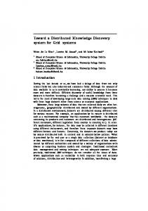
Following the CTA, data visualizations were developed to help improve operator performance. These visualizations were based on operator discussions and indications of needs. Usability testing of the visualization using a student population was performed to identify potential areas of improvement for the visualizations. COGNITIVE NEEDS ANALYSIS APPROACH This research employed task diagrams and knowledge audits to perform a CTA on three desks within power utilities: Generation Desk, Balancing Authority Desk, and Reliability Desk. The Generation Desk is primarily responsible for ensuring that all components of a utility (or a region within a utility) are functioning within normal bounds. If elements are to be taken offline for maintenance, transmission operators (TOs) man the Generation Desk and are responsible for ensuring that this information is forwarded to allow for that work to take place. TOs are primarily concerned with the operation of the generators, lines, buses, etc. The Balancing Authority (BA) Desk is responsible for ensuring that adequate generation capability is available across all components, in some cases for buying and selling of power reserves, and for monitoring the entire utility performance from a higher perspective. The Reliability Desk is responsible for monitoring the utilities region as well as the other regions in the US. Reliability Coordinators (RCs) perform case studies on identified contingencies throughout the day to understand the impact of system changes within and outside the utilities footprint. Decisions on mitigation plans for high priority contingencies are developed with input from TOs and BAs. Figure 1 provides a graphical representation of how the desks are related. The information that is available at a lower level desk is available to a higher-level desk.

Balancing Authority Desk

Generation Desk  • • •

Individual Generators,  busses, lines, switches,  etc.  “Regions” within the  utility (depending on   utility size)  Is the equipment 

• • • •

Entire utility area  monitoring  Assessment of reserves  (buying or selling of  power)  Is the system following  the projected load?  Which equipment should  be brought online or  shut down based on the  current situation? 

Reliability Desk • • •

•

Entire power grid  monitoring  Contingency analysis  based on current system  state  Does a contingency with  the utilities region  require a detailed plan  of action?  Does a contingency  outside of the utilities  region require action? 

Figure 1. Interrelationships of the desks within electric utilities Interviews were scheduled with current operators at three utilities (Tennessee Valley Authority—TVA; Southern Company—SoCo; and South Mississippi Electric Power Association—SMEPA). For each desk present at each utility, four operators were interviewed, with the exception of SMEPA in which one operator per desk was interviewed. Semi-structured interviews were conducted to identify the decision points for each desk task, identify information 46   

used to make appropriate decisions, clarify how information was integrated to understand system status, and identify perceived vulnerabilities in the system. Interviews were paused or stopped when operators needed to perform job functions. If the interruption required action on the operators’ part, they were asked to step back through the event and describe what had occurred. Interviews typically occurred spanning the shift changes (6 am and 6 pm). Therefore, two researchers met with two different operators from 3:00 – 5:00 am/pm and 7:00 – 9:00 am/pm at each desk within three utilities. This was done to limit our time interrupting normal operations and to ensure that we obtained a representative sample of how individuals performed the task. Because different utilities have different set ups, job functions are not necessarily equivalent at the same desk. For example, at Southern Company there were only two desks (Reliability and Balancing Authority), though the Balancing Authority Desk performed many of the operations of the Generation Desk. At South Mississippi Electric Power Association, there were also two desks, the Reliability Desk and the Generation Desk, though the Generation Desk performed many of the functions of the Balancing Authority Desk. Table 1 provides participant demographics for this study. As can be seen in the table, operators varied in age and in experience level. Most operators were Caucasian, and only one operator indicated English was their second language. From these interviews the following generic task diagrams were developed. Table1. Participant demographics Age 50 37 45 43 44

Gender Male Male Male Male Male

47 Male 46 55 24 31 57 39 45 41 48 39 32

Male Male Male Female Male Male Male Male Male Male Male

Ethnicity Caucasian Caucasian Caucasian Caucasian Caucasian AfricanAmerican Caucasian Caucasian Caucasian Caucasian Caucasian Caucasian Caucasian Caucasian Caucasian Caucasian Caucasian

Total Experience in Experience in this Position Control Centers System Operator / Reliability Operator 5 yrs 5 yrs Reliability Coordinator 6 mo 14 yrs Balancing Authority Real-Time Operator 1yr 10 yrs System Operator 1 yr 19 yrs Specialist Reliability Analyst & Operator 4 yrs 14 yrs Title

Specialist Reliability Analyst & Operator

3yrs

28 yrs

Balancing Authority / System Operator Transmission System Operator Transmission Operator Balancing Authority Transmission Operator Senior Balancing Authority Reliability Coordinator Reliability Coordinator Transmission Operator Power System Operator Reliability / System Operator

4 mo 7 yrs 1 yr 1 yr 7 yrs 7 yrs 1 yr 4 yrs 8 yrs 6 yrs 6 yrs

4 mo 20 yrs 4 yrs 1 yr 7 yrs 8 yrs 7 yrs 8 yrs 8 yrs 17 yrs 6 yrs

47   

FINDINGS The two-hour semi-structured interviews with operators were transcribed and analyzed by analysts that performed the interviews. From the transcribed logs, generic task diagrams for each desk were developed. Knowledge audit details were also extracted and are presented below. It should be noted that operator preferences in how they complete the steps in the task diagram are somewhat variable. The knowledge audit details provide a summary of all informational sources identified by operators to successfully perform their tasks, though all operators may not use all informational sources identified. Generation Desk The task diagram for the Generation Desk is provided in Figure 2. Five generic tasks were identified: changeover, region/utility status, workload/job scheduling review, switch-out lines review, and changeover. Details for each task are provided below. The purpose of the changeover is to gain an overall understanding of the current system status, get an update on any events or occurrences from the previous shift, and to inform on-coming transmission operators (TOs) of continuing events that would impact their shift. It is critical that off-going TOs inform on-coming TOs of anything that has changed the system from the last shift (e.g., a unit/generator coming off line). Logs are a primary source of information that provides details on actions taken during the shift. TOs determine, based on the frequency of the event (is it a common or rare event), what type of information to enter into logs. Most of the changeover takes the form of verbal communication between the off-going and on-coming operators. Offgoing TOs will provide case study data, if it exists, discuss alarms, discuss holds, and any other additional information that would impact the use of or shut down any element of the system. The changeover process takes approximately 30 minutes to 1 hour. Therefore, TOs typically come on shift 30 minutes prior to the official start of their shift (6 am or 6 pm).

48   

Changeover 

Region /  Utility Status 

Changeover  Workload /  Scheduled Job  Review 

Switch‐out  Lines Review 

Changeover: 

Region/Utility Status:

•

• • • • • • •

System changes 

Workload/Scheduled Job Review:  •

Logs  One‐line diagram   Voltages  Alarms  Contingencies  ACE  Load trend

Element functionality 

Switch‐out Lines Review: • • •

One‐line diagram  Holds  Caution orders 

Figure 2. Task diagram and knowledge audit information for the Generation Desk After logging into the system following the changeover process, TOs unfailing said they perform a scan of data to obtain a “big picture” of the system, or their region of the system. Logs are again frequently used to review past actions, particularly if the TO has been off for a couple of days or for a week. This is where the details of the actions taken on the previous shift are recorded. The one-line diagram, often called the board, is also viewed. This diagram provides a representation of the system with various colored lights indicating whether a unit is on, if there is a hold, if there is a problem with an element, etc. Also, it contains the voltages for elements in the system. TOs will become familiar with company desired voltage ranges for equipment and normal operating conditions. Voltages are checked to determine what elements may not be functioning under normal conditions. An alarm summary is also viewed. Alarms have various levels and are often presented based on priority level, with the highest-level priority alarms having a designated color (red), followed by yellow, then white (though these color indicators may vary slightly across utilities). Auditory signals are also used for high-level alarms to increase perception of the alarms by TOs. A list of contingencies may also be viewed to determine event sequences should any single element of the system go down. Contingencies, without fail, are listed by priority, with highest priority contingencies being listed first. Contingencies that would have an element running at greater than 95% of its capacity are required by NERC (North American Electric Reliability Corporation) to have mitigation plans developed in the event that they occur. Depending on the likelihood of that contingency occurring, preventive actions may be implemented (such as bringing on another generator, reducing generation at a specific plant, opening or closing lines to redirect power flow, etc.). The likelihood of the contingency is an experience-based determination. As with most systems, 49   

each system has areas that are less stable or more prone to events. If the contingency is related to a known problem area, preventive actions are more likely to be taken. For common contingencies, some utilities have documented solutions for mitigating that contingency while other utilities rely on case study application for the development of appropriate mitigation plans. While the TOs are responsible for developing mitigation plans, they work with their reliability coordinators (RCs) to identify the most effective, least disruptive mitigation plan (meaning the plan that has fewer impacts on other areas of the system). Because there are a large number of elements in the system, there are multiple solutions to each contingency. All actions taken on the system will impact other areas of the system. Therefore, the RC will review the mitigation plan developed by the TO to ensure that the actions taken to circumvent one contingency will not place undo stress on the system at another location. Other tools used to obtain the big picture of the current system state are the ACE graph (is the ACE within normal regions), load trend or load number data (is the load above or below forecasted load, is load increasing or decreasing), and current weather situations (what is the temperature, potential for storms or wind). The third step in the task diagram is viewing workload/scheduled jobs. After understanding the state of the system, a review of scheduled jobs allows the operators to make a determination of whether or not the job should be completed as scheduled (e.g., an unexpected occurrence that disabled the element already, unexpected occurrence requires that element to be functional for power flow due to damage elsewhere, if one of two lines servicing an area are already down then the TO will not allow the second line to be taken down, etc.) or if there are holds on lines. If the utility is currently under- or over-generating, then the TO will need to begin determining which generators to engage or release to address that need. The Balancing Authority will make the call as to which generator to address, but the TO should be looking at possibilities as well and the effects on those parts of the system that are less stable or where there are job being performed. Checking the switch out lines is related to the previous step. TOs will view the one-line diagram and determine which lines to open or close to direct power where it is needed within that utilities footprint. This decision is made based on safety and whether there is a need to drop load. Lines cannot be opened if there are workers on that line. Hold orders are listed in the system and indicate that maintenance is being performed on that line; that line is also shaded orange on the one-line diagram. Caution orders are lines that are in services but set to trip under specific load conditions to protect the equipment; indicated by yellow shading. Temporary alternative permits indicate that there is something abnormal on the line. TOs will end their shift by performing the changeover task for the on-coming operator. Balancing Authority The task diagram for the Balancing Authority is provided in Figure 3. Five generic tasks were identified: changeover, system status, interchange schedule, short term dispatching/forecasting, and changeover. Details for each task are provided below. 50   

System  Status Changeover 

Changeover 

Short Term  Dispatching /  Forecasting 

Interchange  Schedule 

Interchange Schedule: Changeover: 

System Status:

•

• • • • • •

System changes 

• • • • •

Logs  Weather  Load profile  ACE  Contingencies  EMS (Emergency  Monitory System)

Interchange schedule  Weather  Reliability desk instruction  Load profile  Resource list  f l d

Short Term Dispatching/Forecasting:  • • •

Load profile  Resource list  TOs 

Figure 3. Task diagram and knowledge audit information for the Balancing Authority The changeover process is the same at this desk as it was for the Generation Desk. The system status check is also very similar in that the objective is for the operator to gain an understanding of what is happening within the entire utility footprint as a function of load. The function of this desk is to make sure that sufficient generation capacity exists for the load demand and to buy or sell power as needed, depending on the utility. The load profile is critical to determining current system status. The load profile is a trend that plots forecasted and actual load, allowing operators to see very clearly if the utility is over- or under-generating. A screen listing resources, current usage levels, status (on or off line), and capacity levels is also used to determine what resources are available and working. ACE is again monitored to ensure that the system is functioning. Contingency analysis pages are also viewed to assess if lines will go on or off line. The EMS (Emergency Monitoring System) is also monitored to view systems status and any changes in the system. The interchange schedule is where operators can view the buying and selling of power. Depending on the load profile, operators at this desk will determine if there is the need to buy or sell power. During ramp up (when load is increasing) power reserves will be utilized, reducing the ability of the utility to supply their own power economically. During ramp down (when load 51   

is decreasing) reserve power will begin to increase and economical forms of power will become more readily available. The decision to buy power when you have reserve power is dependent upon the type of reserve power available and the utility. For example, for some utilities gas power is one of the most expensive types of power to use. Therefore, it may be more economical to buy power from a surrounding utility than to utilize these power sources. Other utilities, however, have fossils as their most expensive power sources. The economics of the power sources is driven by the location of the utility and the number and type of generating plants. The decision to buy or sell power is based on the load profile. Weather also plays a major role in the decision to buy or sell power. Heat buildup on the earth’s surface dissipates quickly during clear weather, resulting in a reduced load later in the day and into the night. However, when the sky is cloudy, the heat is trapped beneath the clouds and results in an increase in load demands. The load forecast for the day is based upon weather forecasts, though the accuracy of the forecasts is marginal. Therefore, operators need to be cognizant of current weather conditions and make buying/selling decisions, appropriately. When needing to buy power, the utility will place an order on the interchange and marketers will “shop” at the other utilities to find the best deal for the power. When selling power, the BA will determine the appropriate price based on cost to generate the power and the marketer will sell to utilities as needed. As will be seen in the discussion of the Reliability Desk, these transactions can be disrupted due to equipment loading; therefore, these transactions occur throughout the day. Typically, operators “run the numbers” at the bottom of every hour for the next hour, meaning they determine whether or not they need to buy or sell load, and the appropriate price for power reserves. Viewing non-conforming loads is also critical. Non-conforming loads are loads associated with large industries that have nonuniform power ramp-up and –down requirements throughout the day. Operators can view load profiles and estimate when these loads will increase and decrease (as they are somewhat predictable—meaning if these loads have been low they will increase and if the loads have been high they will decrease). Integrating information from the load profile and the non-conforming load profile will dictate if additional reserves will be available (when the non-conforming loads are ramping down) or if additional power will be needed (when the non-conforming loads are ramping up). Short-term dispatching and forecasting are the last major activities that are performed by BAs. These activities are related to adjusting generation schedules based on specific time frames. Short-term dispatching is related to making decisions based on the current situation, the next hour, or two hours out. Decisions about which generators to bring on line or to bring down are all based on economics, as discussed above. Cheaper energy sources will be tapped first, and expensive energy sources will be brought down first. Depending on the utility, short-term dispatching and long-term forecasting may be done by the same or different operators. Shortterm dispatching activities require interaction with TOs to assess functionality of current units within the system. For example, if the BA is planning on using a recently down unit to redispatch power, then a discussion with the TO (or confirmation) about the units availability will occur. Again, weather will play a role in how, when, and where power is re-dispatched. For 52   

long-term forecasting, BAs will consider expectations for the rest of the shift, for the next shift, and for the following day. Forecasts will have already been developed; therefore, BAs will review these forecasts, look at current load demands and weather patterns, and make adjustments accordingly. Changes to schedules for unit usage are likely based on BAs projections. As before, the BA ends their shift by performing a changeover. Reliability Desk The task diagram for the Reliability Desk is provided in Figure 4. Four generic tasks were identified: changeover, grid status, case studies, and changeover. Details for each task are provided below. Grid  Status Changeover 

Changeover 

Case Studies

Changeover: 

Grid Status: 

Case Studies:

•

• • • • • •

•

System changes 

Logs  Weather  Contingencies  RCIS  TLR  Interconnect flow  diagrams or trend  graphs 

• • •

On‐line and off‐line  applications  State estimators  Operating procedures  Strategy documentation  BA TO d h RC

Figure 4. Task diagram and knowledge audit information for the Reliability Desk The changeover process is the same at the Reliability Desk as for the other desks. Again, all reliability coordinators (RCs) indicated that they perform a scan of numerous data streams to obtain an assessment of the grid status. Unlike the previous two desks, RCs are concerned with the entire power grid, particularly those utilities and regions that are adjacent to a particular utility. A critical informational source is the Reliability Coordinator Information System. This system is used by all RCs to send information about a utility that the entire industry needs to know (such as the loss of generation or transmission capability). Transmission Load Relief (TLR) pages are also critical as they indicate what areas of the grid are currently overloaded. A TLR is a request by a utility to redirect energy distribution to reduce load on elements within a utilities footprint. An Interconnect Flow Map is used to provide a quick view of flows across 53   

interconnects. An RC will be able to easily see which direction energy is flowing (east to west, north to south) and the magnitude of that flow. This map can also identify flow direction and magnitudes across specific utility regions. A utility region may be comprised of several utility companies or a single utility company depending on the set up. Interconnect trend graphs may also be used in place of Interconnect Flow Maps to describe energy flows. The alarms page is also used by the RCs, though not to the extent of the TOs. Logs are also used, in the same manner as the two previous desks. Contingency pages, for the utility and for the entire grid, are likely the most critical pieces of information for RCs. These contingencies describe effects that would occur if a single element in the system were to go out of service along with the magnitude of those effects (lines would be working at specific capacity levels—can be greater than 100%). The Reliability Monitor, or similar screen name, is a snap shot of the utilities system that is updated every few minutes and is used to update contingencies. Frequency is also monitored continuously as large swings in the frequency of the system are indicative of problems. Normal ranges for frequency swings in the US are from 59.92 to 60.04. Anything larger would result in RCs looking into the systems and grids to determine the cause of the frequency shift. Case studies are the primary task of RCs. As alarms and contingencies are identified, RCs will run case studies to determine mitigation strategies and determine if they meet utility requirements. Depending on the utility, these requirements may be structured differently; however a common thread is to deal with those contingencies that result in the largest effects on other components in the system. Several on-line and off-line application tools exist that allow RCs to input data from the current system state and test various strategies to address these contingencies. Much of the knowledge for addressing contingencies is learned on the job. Knowing what resources are located where, which contingencies are common, effective strategies for past events, etc. are all used to help RCs make their decisions. For novice RCs, operating procedures for dealing with categories of contingencies exist. In some instances, the most recent or common mitigation strategy is documented to provide a starting point for problem solving. Further, one-line diagrams are available that show the relationship of resources to the areas in question. As contingencies develop, time stamps for implementation of the strategy are provided. For example, if a specific line is to trip and the result in an overload on another line, it will be indicated that mitigation must be implemented within 5 minutes to prevent equipment damage or further contingencies. Depending on the situation, high priority contingencies can have an implementation range of 5 to 30 minutes after occurrence. Discussions with TOs, BAs, and other RCs are also critical and used to help in the development of mitigation plans. These individuals are used to verify that the information being received on an alarm or potential contingency is correct, and to develop effective mitigation strategies. Unlike the Balancing Authority Desk, RCs do not make decisions based on economics. Their decisions are based on ensuring that all entities in the grid receive sufficient power to function (homes, hospitals, schools, etc.). There are three basic mitigation plans that RCs will employ: redistribution (increase or decrease generation), reconfiguring the system (opening and closing lines to force power where it needs to go), and load shedding (cutting power to areas of the systems). While 54   

the specific type of plan implemented varies based on RC preferences, load shedding is a last resort. Only if no other mitigation plan works will RCs implement load shedding. It should also be noted that RCs are the final decision makers in mitigation plans. While TOs or BAs may contribute to the development of mitigation plans, RCs will ultimately decide which plan to implement. A difficulty in document effective mitigation strategies is that the system is constantly changing. Therefore, a strategy that worked for one scenario may not work for a similar strategy, based on which lines are open or closed locations of on-line generators, load demands within and outside the utilities footprint, etc. As before, the RC ends their shift by performing a changeover. Common Issues with Task Performance Every operator, without fail, indicated that weather instances were the most influential outside force. Thunderstorms, particularly rapid moving storms, pose significant threats as they have the potential to short out lines. The storms may be accompanied by strong winds that can result in line trips or downed lines, and can result in loss of power to large areas of a utility (such as an entire city). Knowing the unstable areas of the system can assist in predicting some of the instances or events that will need to be dealt with during and following a storm. However, there is no way to know the exact impact of a storm on the system. Also, as mentioned earlier, specific weather conditions (cloudy weather) have predictable impacts on load and operators need to learn those impacts and begin to anticipate them. As a result, video streams of outside conditions are helpful. However, some utility footprints are so large that it makes it difficult for operators to know exact weather conditions across the entire footprint. The use of weather maps is necessary and provides timely information to assist in preparing for potential weather related events. Every operator also indicated specific issues associated with seasons. During the summer, loads are high due to increased usage of air conditioners. However, there is only one peak in load that occurs around 3 pm that operators have to plan for. During the winter, there are two peaks in load, one in the morning when the footprint area “wakes up” (between 6 am and 9 am) and one in the evening when lighting and heating units turn on. Therefore, operators are trying to predict system performance across two peaks increasing the difficulty of their job task. Operators indicated spring and fall as the most likely time for unusual occurrences. This is due to maintenance schedules on equipment. Often a large number of units or elements in a system will be scheduled to be down during these seasons. However, spring and fall have some of the worst weather patterns and weather tends to be more unpredictable. If events occur during these seasons, there is an increased probability that the system cannot account for these changes due to unavailability of resources. Missing information across systems is also problematic, particularly from a reliability standpoint. The reason for the missing information in one-line diagrams (such as amps, wattage, voltage) is 55   

debated. Some operators believe that a specific utility has simply decided to not release that information, which requires RCs to call those utilities to obtain the information when contingencies or events occur that are associated with those elements of the system. Other operators believe it is the lag in the updating of system models. Regardless, the incorporation of incomplete data sets hinders performance and can delay timely action to events. The delay in updating system models is also problematic. While a utility will likely have updates to their systems updated automatically, changes to other utilities typically occur once a year. This can lead to incorrect information being presented. For example, one RC illustrated an instance where the model showed a line with two open breakers open, yet there was a reading for energy flow across that line. Instances such as this are a common occurrence, and operators are often calling individuals both within and outside a utilities footprint and finding misinformation has been provided to the control centers. As the systems are dealing with electrical equipment, there will be failures, and some level of information error is expected. However, more frequent updates to system models could relieve some of the wasted effort in verifying information that is based on an incorrect system model. During the interviews, it was discovered that a minimum of approximately 10 minutes is needed to understand an event and to take effective steps to rectifying that situation. During sudden and unexpected events, it is likely that operators will not have 10 minutes with which to make decisions. Operators rely on their knowledge of the system(s) to begin implementing actions to correct event occurrences. It is necessary to understand how operators make decisions under these conditions and are given practice in performing under these types of situations. When pressed for answers to describe how they make decisions under these conditions, operators typically responded that they simply try what has worked in the past and then deal with the effects of that decision, hoping that at some point sufficient time will be bought to approach the problem using standard protocols. It is possible that events can occur in such a way that there is insufficient time for individuals across the desks to discuss the situation and agree on a plan of action. Again, practice on these types of situations is needed Though most operators indicated that they were satisfied with their training, simulator training was repeatedly mentioned as an area for improvement. Each utility has a simulator and uses it routinely in training. However, differences in screens, tools, and data presentation between the simulator and workstations make the simulator less effective. Also, many operators indicated that the simulators were often inoperable, preventing simulator training. VULNERABILITIES OF THE POWER GRID INFRASTRUCTURE Operators were asked if they believed the power grid is vulnerable to intentional attacks. With the exception of a single operator, all answered yes, and most indicated surprise that it has not happened yet. The remoteness and vastness of the infrastructure are two of the common reasons for this vulnerability. For example, it is not possible to patrol thousands of miles of gas and 56   

power lines, thereby making it easy to disable the transmission capabilities of the system. Further, most indicated that there are “key” points in the infrastructure that if attacked, would render the grid powerless. Operators were split roughly 50/50 as to which is more important in maintaining: generation or transmission. However, it was acknowledged that transmission could be repaired faster than generation capabilities. Most operators indicated that random outages or downage would be indicative of potential intentional attacks. However, if the events were concentrated in specific areas where there is no reason (such as weather related events), intentional attacks would be possible causes. Cyber attacks to the grid would be more difficult to accomplish, though certainly not impossible. The redundancy in the systems, in the forms of various data streams providing information that will essentially tell the same story, make interfering with a single piece of data ineffective. Also, the data would need to be “infected” for all utilities, otherwise other operators would “see” the attack occurring. Attacks that could potentially occur on the power grid are not always easy to classify. Possible attacks to the power grid system can be classified as either being physical or software related. Physical attacks could be attacking remote substations in order to disrupt the power flow onto the grid. From the software point of view, irregularities as to the control that operators would normally have could be potential indicators that an attack is then occurring. Also, if the operator monitors and the control center monitors are showing completely different readings then it could be a potential sign of software foul play. There are, however, common themes that the operators agreed would make them question if something irregular was occurring. The first theme would be the weather. It is expected that during certain weather conditions (heavy thunderstorms, flood season, etc) that things like power outages and downed lines will occur. These are normally seasonal events so operators are used to seeing various drops across their systems. Drops that occur during non-seasonal times will normally get the attention of operators. Sudden frequency drops, as well as overall power loss on the grid, will immediately get their attention. They will try to minimize any cascading effects first and then try to determine what happened. Most substations also have remote cameras and will be used initially during investigations. Other workers may be called to go and investigate lines and substations to determine what has occurred. Another theme that would alert operators would be any type of serious problems that seem to happen in close conjunction. Normally, all power systems have various protection schemes that will take effect whenever problems occur to limit the damage that could potentially occur to both the personal company system as well as the grid. Problems that seem to circumvent these schemes always make the operators think that it may be something non-natural causing them, raising suspicions of foul play. A sudden change in the value of the ACE would also alert operators that something suspicious might have occurred. Once again, during bad weather conditions these types of system behavior are expected but during good weather conditions these are the types of grid behavior that may be warnings of sabotage. 57   

Several of the operators offered suggestions for the issue of man-made attacks on the power grid. While it is not always possible to monitor all of the substations, it is possible to speed up the action taken. One way is to give the operators additional training to what are gross irregularities in the system. The area representative of Homeland Security could be brought in to give a brief talk to the operators. Topics covered could include any serious concerns over what areas are potential targets, new groups making threats to the grid, etc. This could help to make operators more alert to irregularities that they may encounter. Another suggestion was to install into a phone line to the area representative of Home Land security. This line would be for the operators to use whenever they believe a serious threat may be occurring, whether or not their employers believe otherwise. The operators would of course be trained to not abuse this line. Beefing up the number of security cameras at remote sub stations as well as having a roaming security officer for all stations are other preventative measures that operators suggested. VISUALIZATION DEVELOPMENT Based on results from the CTA, preliminary visualizations were developed to supplement current operations. Some visualizations were modifications of current displays to improve information synthesis, while other were new visualizations based on operator comments. These visualizations should be viewed as initial steps to improving situational awareness during task performance. Continued research on modifications and development of additional data visualizations would require additional in-depth analysis and study. Four visualizations were developed by the research team and related to alarms, contingency analysis, load profiles, and synthesis visualizations. Screen shots of each visualization are provided in Figures 5-8. A brief description of each visualization is also provided. Alarm Visualization The alarm visualization is a supplement to current alarm displays. As mentioned in previous sections, alarms are a common occurrence. For larger utilities, there is currently no way to organize alarms based on region. For example, TVA transmission operators only monitor a portion of the TVA utility footprint. However, the alarms page displays all alarms for the entire utility footprint. Therefore, it takes significant training and experience to recognize when an alarm is associated with a specific region of the utility footprint. To help reduce the uncertainty associated with the region the alarms are associated with, a column was added that identifies the region (titled “sector”) in which the alarm is occurring (Figure 5). The addition of this column will help operators respond quicker to the alarm, particularly to those that require immediate action on the part of the operator. For smaller utilities, this may not be necessary, though likely those footprints can also be divided into fewer regions and new operators would benefit from knowing where the alarm is located. This could also potentially improve performance in developing plans for dealing with the alarms. It would help reduce the uncertainty of what resources are located near the alarm that could potentially be used to offset or eliminate any 58   

disturbance caused by the alarm (e.g., the loss of generation or transmission capacity). Additionally, a column titled “routine-ness” was added to further help new operators understand which alarms are common and which are not. While all alarms are color coded to assist operators in understanding the importance of the alarm, some alarms are more frequent because of limitations or weaknesses in the system. The addition of a column that identifies how common the alarm occurs is thought to provide operators with further information on the severity of the alarm. Further, rarely occurring alarms may require additional time to develop a strategy for dealing with any impacts the alarm has on the system. If operators are informed of the routine-ness of the alarm, they can be better prepared to deal with that alarm.

Figure 5. Alarm page visualization representation. Contingency Analysis Visualization The second visualization was an extension of the contingency analysis page used by the reliability desk. Currently, there is a time frame specified for reliability coordinators to develop contingency plans for identified critical potential events (events that would have a significant effect on this system if a component was found to fail). As with alarms, these contingencies are color-coded and those that have the highest potential for impact are listed first. Additionally, in the current contingency page there is an identified time limit associated with each contingency that represents the amount of time the system has before there is an overload if the contingency were to occur. For the visualization, a color fill-in timer was developed to assist reliability coordinators in visualizing how much time remains for developing the contingency plan (Figure 6). Within the visualization, a bar graph is used to show how much total time is available to deal 59   

with that contingency and fills up as time elapses. When only a few minutes remain, which is associated with the total time available), the bar graph changes color from green to red to notify reliability coordinators of the need to develop their plan. For seasoned operators, the benefit of the visualization is a reduction in workload in remembering when the contingency was presented, thereby allowing the operator to focus on developing a contingency plan or performing other aspects of the job tasks. For novice operators, this visualization can be used as a training tool to assist in plan development (i.e., how long will it take to develop specific plans). Workload is also reduced for these operators as for the more seasoned operators.

Figure 6. Contingency page visualization representation Actual/Project Load Visualization The third visualization is an enhancement of the load profile information currently being displayed at each utility we visited. Different utilities used different means to present this information. However, many utilities and operators preferred to see a trend in predicted and actual load data. Load data is critical for the balancing authority, who must ensure that sufficient resources are available within the utility or can be purchased from surrounding utilities to fulfill the power needs of the utility footprint. This information is used to determine the amount of power to be bought or sold and associated prices. The enhancement to the current display adds rollover capability to a single display, allowing operators to view simultaneously what the actual and predicted load is at any given point in time. While this information is available in a separate location, combining this information reduces the need for multiple displays to be viewed. 60   

Information is thereby condensed, reducing search and synthesis time. The proposed solution is that for the current hour, the values for the current and predicted load would remain on the screen and update every hour. Operators could use their mouse to roll over the next hour predicted load curve to obtain that data immediately. The purpose of this enhancement is to help increase operators’ awareness of the system status and assist in decision-making.

Figure 7. Projected and actual load visualization representation Synthesis Visualization The final visualization is a synthesis page. There are four key pieces of information that are used by all operators during the course of the workday: ACE, frequency, load, and voltage. Operators are constantly monitoring these key indicators to determine if they are increasing, decreasing, or holding steady. Rapid changes in any of these indicators alerts the operators to take measures or to be prepared to take measures to ensure the viability of the power grid. Therefore, a visualization was created that provides a rapid look at the current values and trends of these critical pieces of information. Color-coded arrows are used to provide information on the speed and direction of data change (Figure 8). For data that is holding steady, green arrows pointing to the right are used. For data that is increasing or decreasing at a “slow” or “normal” pace, yellow (or orange) arrows are used, and red arrows are used to denote data that increases or decreases at a rapid pace. Additionally, the current values for these data are provided, along with a clock, to assist in decision-making. The purpose of the visualization was to provide a rapid check on critical system status information to facilitate situational awareness and decision-making. This visualization would be of benefit to both experienced and novice operators. 61   

Figure 8. Synthesis page visualization representation USABILITY TESTING USING MSU STUDENT POPULATION Approach Usability testing of the developed visualizations and the database interface were conducted to improve design and gauge the usefulness of these entities. Eight students, 7 males and 1 female, from the Mississippi State University (MSU) student population were recruited to serve as test subjects for this study. Participants first received a verbal and written description of the project, its objectives and procedures, and signed informed consent documents prior to data collection. Participants were shown screen shots of each visualization and the database interface one at a time. Order of exposure to the screen shots was randomized across participants. A brief description of the visualizations purpose was provided in written form (for example, this visualization shows an event that may occur and the time required to address that event before power loss). Participants were allowed to view the visualization for as long as needed and then answered questions pertaining to the visualization or database, after which they completed a short usability questionnaire. A copy of the usability instructions, visualization description, tasks, and usability questionnaire are provided in the appendix. Repeated measures ANOVA was used to determine if significant differences existed in total usability score and normalized usability dimension score across visualizations (details on how normalized usability dimension scores were computed are presented below). Where significant findings were identified, Tukey’s HSD post hoc analyses were conducted. All results were considered significant at an alpha level of 0.05. Data analyses were conducted using SAS 9.1 statistical software

62   

Results Table 2 and Figure 9 provide descriptive statistics for the usability ratings for each visualization. As can be seen from the table and figure, the load and alarm visualizations were rated as the best, with the synthesis visualization being rate the least useful. In general, the males tended to rate the visualizations more usable than the female participant, though statistics were not performed to determine if this was a significant difference to the low number of female participants. Table 2. Mean usability ratings for the visualizations and database Female Mean Male Total Usability Mean Rating Rating Rating Visualization Rating (n = 8) (n = 1) (n = 7) Alarm

107.50

5.02

4.18

5.87

Contingency

71.25

3.41

2.95

3.86

Database

82.30

3.94

3.42

4.47

Projected/Actual Load 111.00

5.84

5.84

5.84

Synthesis

3.06

2.32

3.81

Females

7 6 5 4 3 2 1 0

S yn th es is

D at ab P as ro je e ct ed /A ct ua lL oa d

C on tin ge nc y

Males

A la rm

PSSUQ rating

68.88

Visualization

Figure 9. Mean usability ratings for the visualizations and database

63   

Mean

Visualizations were found to have statistically significant different total usability scores (p = 0.0004) (Table 2). The load and alarm pages were found to have significantly higher usability ratings than the contingency and synthesis visualizations. Both visualization and dimension were found to significantly affect usability dimension score (both p’s < 0.0001). There were seven usability dimensions considered: learnability, satisfaction, design/layout, ease of use, errors, functionality, and outcome/future use. Because each dimension had a different number of questions associated with it (e.g., three questions related to learnability, two questions related to error, etc.), data were normalized prior to analysis. The total points earned were divided by the total points possible. Therefore, values were a number between 0 and 1 and represented the percentage of points earned. Figure 10 provides the results of the usability dimension analysis. As can be seen by the figure, the synthesis and contingency visualization earned significantly less dimensions scores than the alarm and projected/actual load visualizations. Also, the error usability dimension was rated lower for all visualizations than the other dimensions. There was not dimension by visualization interaction effect.

Percent Score Earned

1 0.8 0.6 0.4 Alarm Database Synthesis

0.2

Contingency Projected/Actual Load

Satisfaction

Outcome/Future Use

Learnability

Functinality

Errors

Ease of Use

Design/Layout

0

Usability Dimension

Figure 10. Usability dimension effects by visualization SUMMARY There are three primary desks within electric utilities that perform different functions (transmission operators, balancing authorities, and reliability coordinators). There exists a high level of uncertainty associated with these desks as the changing state of the power grid changes how operators can successfully deal with changes in the system status. A number of data sources 64   

are used in the performance of each task, and the focus on the specific data sources is different for each desk. These desks must work together to ensure that the power grid remains viable not only for a specific utilities footprint, but for the entire power grid. Discussions with operators revealed that increased focus on training, in particular simulations, would improve operator performance and situational awareness. The power grid is vulnerable to both man-made and natural attacks. Operators debate the source of that vulnerability. The elimination of generation capacity as well as transmission capacity can create different levels of damage. It was indicated that man-made attacks focusing on transmission capacity could be extremely detrimental and immediate. Further concern should be given to this area of power grid protection due to the inherent vulnerability and potential for immediate impact that has been highlighted. Visualizations were developed to assist in decision-making capabilities. These visualizations primarily focused on enhancing current visualizations to minimize the need to review multiple sources of data. Usability testing of these visualizations by a novice population indicated that further refinement is needed for specific visualizations. However, in general, operators were able to use the visualizations effectively, particularly those associated with the projected/actual load and alarms.

REFERENCES [1]. Wickens C (1984), Engineering psychology and human performance. Columbus, OH. [2]. Sanders MS and McCormick EJ (1993), Human Factors Engineering and Design, 7th Edition, New York, NY, McGraw-Hill, Inc. [3]. Barnard, P. & May, J. (2002), Cognitive task analysis, Retrieved June 5, 2002 from the World Wide Web: http://www.mrc-cbu.cam.ac.uk/amodeus/summaries/CTAsummary.html .

65   

Appendix Usability Testing Forms I. Purpose:

Projected vs. Actual Load

The purpose of this page is to provide operators with information on what the projected power load is for the day and what the actual load was for each hour of a 24 hour period for planning purposes (for example: is more or less power needed than planned for, is more or less power needed for the upcoming hour(s), etc.).

Instructions: Use the graph on the computer monitor to answer the questions listed below. Write each answer in the space provided. All points on the graph have curser rollover capability. After answering all questions, complete the usability questionnaire. Questions: 1) In hour 16, what’s the projected load? ___________________________________________________________________________ ___________________________________________________________________________ ___________________________________________________________________________

2) What is the difference between actual and predicted load for hour 6? ___________________________________________________________________________ ___________________________________________________________________________ ___________________________________________________________________________

66   

II. Purpose:

Alarms Page

The purpose of this page is to notify operators of any problems in the power companies system or with any of the power transmission (power lines, substation, breakers, etc.) and generation (power plants) components. For example, if a line goes down, this will be identified on this page to the operator. Information about the location of the alarm and the severity of the alarm (in terms of color) are provided. Higher priority alarms are coded red. The color coding is to help assist the operator in determining the need to address the alarm immediately or is the alarm minor and requires little or no action on the part of the operator. These alarms are for the entire power companies areas. For example, all alarms for the TVA area will be on this page (which is quite a large area from Kentucky to Mississippi to the Carolinas).

Instructions: Use the graph on the computer monitor to answer the questions listed below. Write each answer in the space provided. After answering all questions, complete the usability questionnaire. Questions: 1) For alarm 4, what type of device is being used? ___________________________________________________________________________ ___________________________________________________________________________ ___________________________________________________________________________ 2) What percent of limits is identified for alarm 1? ___________________________________________________________________________ ___________________________________________________________________________ ___________________________________________________________________________ 3) How routine is alarm 5? ___________________________________________________________________________ ___________________________________________________________________________ ___________________________________________________________________________ 4) In what sector is alarm 2 located? ___________________________________________________________________________ ___________________________________________________________________________ ___________________________________________________________________________ 67   

III. Purpose:

Contingency Page

The purpose of this page is to list the critical contingencies identified for the power company’s transmission (power lines, substations, breakers, etc.) and generation (power plants) components. Power companies are required to consider all “n-1” contingencies (what happens if this component will no longer work?). For example, if a power company has 100 components, then for the current state of the system, each component will be simulated to be taken out of working order, one at a time, and the impact on the system assessed. Contingencies are coded (using color) to identify which ones will have significant impacts on the system (causing major outages or overloads). Red contingencies are the most important. Information on the amount of time that the operator will have to deal with the contingency if it occurs is provided. Additionally, the time the operator has to develop the plan to deal with that contingency and submit it is also provided. The first column of the contingency page provides the operator with the time they have to generate a plan. The second column provides the operator with a graphical display of how much of that time has elapsed. The remaining columns provide the operators with the details of the contingency.

Instructions: Use the graphs on the computer monitor to answer the questions listed below. Write each answer in the space provided. After answering all questions, complete the usability questionnaire. Questions: 1) For contingency 3, how long do the operators have to address the problem? ___________________________________________________________________________ ___________________________________________________________________________ ___________________________________________________________________________ 2) For contingency 5, does the operator have less than 5 minutes left to address the problem? ___________________________________________________________________________ ___________________________________________________________________________ ___________________________________________________________________________ 3) For contingency 1, does the operator have more than 5 minutes left to address the problem? ___________________________________________________________________________ ___________________________________________________________________________ ___________________________________________________________________________ 68   

IV. Purpose:

Synthesis Page

The purpose of this page is to provide operators with a general picture of the power company’s system status. The color and direction of the arrows provide information on the direction of change in the information (Is it increasing, decreasing or remaining stable?), and the rate of change (is the information changing fast—red, slow—green). By looking at the direction and colors of the arrows, operators can focus their attention on addressing fast changing information to prevent potential problems.

Instructions: Use the charts on the computer monitor to answer the questions listed below. Write each answer in the space provided. After answering all questions, complete the usability questionnaire. Questions: 1) What does the red arrow for load profile mean for time 20:32:17? ___________________________________________________________________________ ___________________________________________________________________________ ___________________________________________________________________________ 2) What does the green arrow for ACE mean for time 20:32:17? ___________________________________________________________________________ ___________________________________________________________________________ ___________________________________________________________________________ 3) What does the yellow arrow for voltage mean for time 20:32:17? ___________________________________________________________________________ ___________________________________________________________________________ ___________________________________________________________________________ 4) At time 13:09:45, is frequency increasing, decreasing, or holding steady? ___________________________________________________________________________ ___________________________________________________________________________ ___________________________________________________________________________ 5) At time 16:24:07, what is increasing? ___________________________________________________________________________ ___________________________________________________________________________ ___________________________________________________________________________

69   

V. Purpose:

Database

The next 5 screen shots deal with a database interface. The purpose of this database is to provide operators with geographical location and temporal (time related) information each sensor in the power company’s system. For example, if a sensor or component (line, switch, breaker, etc.) fails, then the operators can visually see the location of that sensor or component (using a Google-Earth map), surrounding sensors or components that can be used to deal with the failure, and any other location information related to their systems. Additional information on data through that sensor or component for specific time frames can be assessed and analyzed to assist with planning and day-to-day operations. The next 5 screen shots of this database are of different stages of information retrieval and the tasks for each screen shot differ.

Instructions: Use the screen shot on the computer monitor to answer the questions listed below. Write each answer in the space provided. After answering all questions, complete the usability questionnaire. Database (1) Instructions: Use the screen shot on the computer monitor to answer the questions listed below. Write each answer in the space provided. After answering all questions, complete the usability questionnaire. Questions: 1) What sensor is being studied? ___________________________________________________________________________ 2) How do you check the status of a particular station? ___________________________________________________________________________ 3) If line between 18009 and 18131 has gone out of service, how do you get a solution? __________________________________________________________________________ 4) If you needed information for a specific sensor, where would you get it? ___________________________________________________________________________ 5) How do you check the voltage of sensor-1074? ___________________________________________________________________________ 6) What do the pear-shaped icons on the map represent? ___________________________________________________________________________ 7) What is the date and time that the event occurred? ___________________________________________________________________________ 70   

Database (2) Purpose:

See database description.

Instructions: Use the screen shot on the computer monitor to answer the questions listed below. Write each answer in the space provided.

1) How would you get information on a sensor after 12 PM? ___________________________________________________________________________

2) What do the blocks under “Get Capabilities” mean? ___________________________________________________________________________

3) What is the voltage for sensor-289? ___________________________________________________________________________

4) How do you find the solution for Rule 2? ___________________________________________________________________________

5) What is rule 3? ___________________________________________________________________________

6) If rule 3 occurs, what capacitors need to be switched on? ___________________________________________________________________________

71   

Database (3) Purpose:

See database description.

Instructions: Use the screen shot on the computer monitor to answer the questions listed below. Write each answer in the space provided. 1) What is the solution to the problem represented in the screen shot? ___________________________________________________________________________

2) How many stations are represented in the map? ___________________________________________________________________________

3) Where has the real power increased? ___________________________________________________________________________

4) Which voltages have fallen? ___________________________________________________________________________

72   

Database (4) Purpose:

See database description.

Instructions: Use the screen shot on the computer monitor to answer the questions listed below. Write each answer in the space provided.

1) What is the voltage for sensor-289? ___________________________________________________________________________

2) What do the icons on the map represent? ___________________________________________________________________________

3) What sensor is selected for viewing information? ___________________________________________________________________________

4) How do you view a table format? ___________________________________________________________________________

5) How do you view a satellite image? ___________________________________________________________________________ 6) What does “ActPower” stand for? ___________________________________________________________________________

73   

Database (5) Purpose:

See database description.

Instructions: Use the screen shot on the computer monitor to answer the questions listed below. Write each answer in the space provided. After answering all questions, complete the usability questionnaire.

1) What are your offering options? ___________________________________________________________________________

2) What are the lower spatial subset points in space? ___________________________________________________________________________

3) What are the upper spatial subset points in space? ___________________________________________________________________________

4) Is the map in “map”, “satellite”, or “hybrid” mode? ___________________________________________________________________________

5) What do you think RctPower stands for? ___________________________________________________________________________

74   

   

Usability Questionnaire

Strongly Disagree

Post Study System Usability Questionnaire (PSSUQ) (Lewis, 1995) –19 items

Strongly Agree

1. Overall, I am satisfied with how easy it is to use this data/system

1

2

3

4

5

6

7

2. It was simple to use this data/system

1

2

3

4

5

6

7

3. I would be able to effectively complete my work using this data/system if needed

1

2

3

4

5

6

7

4. I would be able to complete my work quickly using this data/system

1

2

3

4

5

6

7

5. I would be able to efficiently complete my work using this data/system

1

2

3

4

5

6

7

6. I would feel comfortable using this data/system

1

2

3

4

5

6

7

7. It would be easy to learn to use this data/ system

1

2

3

4

5

6

7

8. I believe I can became productive quickly using this data/system

1

2

3

4

5

6

7

9. The data/system gives error messages that clearly tell me how to fix problems

1

2

3

4

5

6

7

10. If I were to make a mistake using the data/system, I could recover easily and quickly

1

2

3

4

5

6

7

11. The information (such as online help, on-screen messages, and other documentation) provided with this data/system is clear

1

2

3

4

5

6

7

1

2

3

4

5

6

7

1

2

3

4

5

6

7

1

2

3

4

5

6

7

1

2

3

4

5

6

7

1

2

3

4

5

6

7

1

2

3

4

5

6

7

1

2

3

4

5

6

7

1

2

3

4

5

6

7

12. It is easy to find the information I needed 13. The information provided for the data/system is easy to understand 14. The information would be effective in helping me complete tasks and scenarios related to this data/system 15. The organization of information on the data/system screens is clear 16. The interface of this data/system is pleasant 17. I would like using the interface of this data/system 18. This data/system has all the functions and capabilities I expect it to have 19. Overall, I am satisfied with this data/system

75   

Task III: SENSOR MODEL DEVELOPMENT INTRODUCTION Most of the communication protocols being used in the power system are either vendor proprietary or user developed standards, which is increasing the cost of information exchange between utilities [1]. The lack of standardization of the data exchange mechanism to encapsulate, store, exchange and configure these data sets and the information that goes into the monitoring and forecast, is an impediment for effective decision making. The existence of several inter-dependencies within the power systems makes it vulnerable to cascading of small contingencies into large area outages [2]. Proper information exchange in appropriate time is essential for the prevention of these outages. In recent history, we can find numerous outages which could have been prevented with proper exchange of information among utilities. The proper exchange of information among utilities can be ensured by making all the utilities use the same set of software and communication protocols, so that interoperability between different systems can be achieved. However, this does not seems to be a feasible option because of the multi-billion investments already done by the utilities in infrastructures like training staffs, software and hardware. A more viable option for utilities is to agree upon certain open standards for information interchange without the need to alter their legacy systems. On the other hand, the current system does not provide leverage to security coordinators [2] of a region to monitor the system within his/her region with a single application. The precious time which could have been used to act upon the contingency is wasted just to remove heterogeneity. A central information repository and query system can empower the security coordinator with a tool to act upon contingencies more effectively than ever [1]. Hence it is imperative that strategies for innovative acquisition, integration, and data exploitation technologies be explored for fully interchangeable, timely, and accurate power systems data. The seamless access to real time or near real time power systems sensors data is constrained by varying characteristics (physical/logical) of the sensor networks. Sensor Web Enablement (SWE) provides along with provides a solution to the problems of heterogeneity of data and lack of central repository of the data for proper action in case of contingency [3]. Sensor Web is an emerging technology trend towards achieving a collaborative, coherent, consistent, and consolidated sensor data collection, fusion, and distribution system. It enables to add a sensor dimension to the Internet that allows users to glean meaningful information about the observation via a web browser. As illustrated in the Figure 1, SWE acts as a common interface to the utility data for Security Coordinator, facilitating the seamless access to data and information and reconciles the heterogeneities in various interdependent systems.

   

   

 

Figure 1. Communication of security coordinator with utilities within a region and inter-utility commutation The security coordinator can access the data of all utilities of his/her region from a single client application to decide on the correcting measures for the contingency. In addition to, adding value to monitoring his/her own region, the SWE also enables free communication among security coordinators of the neighboring regions as shown in the Figure 2. The effective communication among security coordinators is vital for preventing contingencies. However, currently the security coordinators are more or less aware of the facts of their region but are ignorant about the neighboring regions.

 

Figure 2. Communication among security coordinators of neighboring regions Figure 3 shows the details of the working of SWE. The characteristics of the current system of sensors like Phasor Measurement Unit (PMU), Potential Transformer etc are described in SensorML hosted by Sensor Observation Service (SOS) while the readings of the sensors are managed in a central repository database of SOS. The AJAX client acts as an interface for the appropriate personnel like Security Coordinator of the region to monitor all the utilities operating in a region irrespective of their internal communication and operational protocol.

77   

   

Figure 3. Detail working of Sensor Web Enablement for power systems SENSOR WEB ENABLEMENT There exist millions of power system sensors which have been employed to monitor numerous parameters like voltage, current, voltage angles etc. But, the data from the sensors is confined to a small group of people generally within a utility. In case of contingency, there is no infrastructure that can be used to share vital information that could be helpful in preventing outages, saving millions of dollars. Sensor Web Enablement can be thought of as a legacy system friendly infrastructure that can be useful for seamless inter/intra-utility information exchange. Sensor web provides the necessary information technology infrastructure on which varied decision support tools could be built (Figure 4). The loosely coupled services in Service Oriented Architecture provide the necessary flexibility for cross domain information integration and querying. Web services decouple objects from the platforms that hold them hostage i.e. web services facilitate interactions among platform-independent objects, which are able to access data from anywhere on the Web. They rely on loose, rather than tight, couplings among Web 78   

   

components. Systems that rely on propriety objects are called tightly coupled because they rely on a well-defined but fragile interface. If any part of the communication between application and service object is disrupted or if the call is not exactly right, unpredictable results may occur. Loosely coupled systems allow for flexible and dynamic interchange in open, distributed Web environments Sensor Web provides a standard method of discovering and accessing the sensor data, so that anyone with internet connection and proper authentication would be able to access the sensor data. According to Kevin A. Delin of NASA's Jet Propulsion Laboratory [5], the "Sensor Web concept enables spatio-temporal understanding of an environment through coordinated efforts between multiple numbers and types of sensing platforms, both orbital and terrestrial, both fixed and mobile. Each of these platforms communicates with its local neighborhood of sensors and thus distributes information to the instrument. The Sensor Web is to sensors what the internet is to computers, with different platforms and operating systems communicating by way of a set of robust protocols." Sensor Web Enablement (SWE) is an Initiative taken by Open Geospatial Consortium (OGC), which have developed unique and revolutionary framework of open standard for communication with the web-connected sensors of all kinds. The main highlight of the SWE is the setting up the communications using Internet and Web protocols, opening up the possibility of Web access. The use of Extensible Markup Language (XML) [6] schemas (formal specifications for structured text) to provide machine-readable metadata makes a great step towards automatic sensor monitoring and control [7]. High level Architecture The SWE initiative is more focused towards development of standard to enable discovery, exchange and processing of sensor observation. The main functionalities of the Power System Sensor web Enablement, powered by OGC SWE include [8]: • Discovery of sensor systems, observations, and observation processes that meet an application or users immediate needs; • Determination of a sensor’s capabilities and quality of measurements; • Access to sensor parameters that automatically allow software to process and geo-locate observations ; • Retrieval of real-time or time-series observations and coverage in standard encodings • Tasking of sensors to acquire observations of interest. The goal of using SWE is to establish a standard communication protocol that can compensate the heterogeneity of internal operational and communicational protocol of power utilities for effective communication in case of contingency. The Power Systems Sensor web facilitates ƒ The description of Power sensors and observation processes with general models and XML encodings through Sensor ML that allows to fully describe them and hence facilitates the dynamic retrieval of their capabilities and quality of measurements ƒ The use of real or near real time data derived from sensors relating to the Power systems sensor networks through Sensor Observation Service (SOS) parameterized observation requests (by observation time, feature of interest, property, sensor); ( see Figure 4) 79   

   

ƒ The dynamic selection and aggregation of multiple sensor systems and simulations in a web services based environment that provides capabilities for discovering systems, observations, and observation processes that meet an application or users immediate needs

Figure 4. Power Systems sensor web enablement provides tools for improved decision making. The following OpenGIS® [www.opengeospatial.org] specifications have been used in the power system Sensor Web development: i. Sensor Observations Service (SOS) - Standard web service interface for requesting, filtering, and retrieving observations and sensor system information. This is the intermediary between a client and an observation repository or near real-time sensor channel, thus avoiding the user to access individual sensor. ii. Sensor Model Language (SensorML) – Standard models and XML Schema for describing power sensors systems and processes; provides information needed for discovery of sensors, location of sensor observations, processing of low-level sensor observations, and listing of workable properties. iii. Observations & Measurements Schema (O&M) – Standard models and XML Schema for encoding observations and measurements from a sensor.

80   

   

SWE Standards Framework The following section describes the SWE specifications used to build the power system sensor web. 1. Sensor Observation Service A Sensor Observation Service (SOS) provides an API for managing deployed sensors and retrieving sensor data and specifically “observation” data. SOS acts as an interface for accessing the sensor characteristics and the sensor data to the rest of world. Instead of communicating with each sensor individually for sensor data, SOS groups sensors into several constellations that can be accessed via SOS [9].There exists variety of sensors from remote sensors to in-situ, fixed to mobile, simple to complex sensors which could be grouped together for a common interface irrespective of the type of the sensor as illustrated in Figure 5 [9].

Figure 5. SOS hides the heterogeneity of sensors from Sensor data consumer

1.1 SOS as an Organizer An SOS organizes collections of related sensor system observations into Observation “Offerings”. Each Observation Offering is constrained by a number of parameters including the following: • Specific sensor systems that report the observations, • Time period(s) for which observations may be requested (supports historical data), • Phenomena that are being sensed, • Geographical region that contains the sensors, and • Geographical region that is the subject of the sensor observations (may differ from the sensor region for remote sensors) The OGC Sensor Observation Service specification defines an API for managing deployed sensors and retrieving sensor data and specifically “observation” data [http://www.opengeospatial.org/standards/requests/32]. Whether from in-situ sensors (e.g., voltage, current, angles etc) or dynamic sensors, measurements made from sensor systems contribute most of the geospatial data by volume used in geospatial systems today. SOS 81   

   

implementation specification defines the interfaces and operations that enable the implementation of interoperable sensor observation services and clients. The SOS is the intermediary between a client and an observation repository or near real-time sensor channel. Clients implementing SOS can also obtain information that describes the associated sensors and platforms. The SOS GetObservation operation includes an ad-hoc query capability that allows a client to filter observations by time, space, sensor, and phenomena as was shown in figure 3 of the Power systems architecture, the different requests such as GetCapabilities, GetObservation, DescribeSensor are handled by the sensor observation service. 1.2 SOS Operation a. SOS-Sensor data Consumer Interaction A sensor data consumer is the application or person interested in sensor data. There may be two kinds of approaches of the data consumer to the SOS, Sensor-Centric approach and Observation centric approach [9]. A sensor-centric point of view would be used if the data consumer was already aware of the existence of particular sensors and wanted to find observations for those sensors. An observation-centric point of view would be used if the consumer wanted to see sensor data from a particular geographic area or particular characteristics or that capture particular phenomena but is not aware of any particular sensors a-priori [9]. Figure 6 demonstrates the sequence diagram that shows a sensor data consumer discovering two SOS instances from a CS-W catalog by using the GetRecords operation. The consumer then performs service-level discovery on each service instance requesting the capabilities document and inspecting the observation offerings. The consumer invokes the DescribeSensor operation to retrieve detailed sensor metadata in SensorML for sensors advertised in the observation offerings of the two services. Finally, the consumer calls the GetObservation operation to actually retrieve the observations from both service instances.

82   

   

Figure 6. Sensor data consumer sequence diagram (adapted from [9]) b. Get Sensor Metadata The power system may have contains sensors that are spatially distributed. In case of contingency, it may be required to get the sensor data of certain sensors to make some critical decisions. Sensor metadata can be retrieved for any sensor that is advertised in an observation offering using the DescribeSensor operation. Each of the sensor characteristics has to be described by the sensor deploying institution (generally utilities) in the form of SensorML. The SOS will return a corresponding SensorML document with detailed information about the 83   

   

sensor. This could be used to filter out sensors that do not have robust error detection and correction or are not accurate enough to rely on by the security coordinator for the decision making. This is an optional step that can be skipped if the consumer has prior knowledge of the sensor. c. Get Sensor Observation This is actual operation of receiving the sensor data. Sensor observations are obtained using the GetObservation operation. This operation supports a query mechanism described below that supports sub-setting the observations that will be returned from a call to GetObservation. GetObservation allows the client to filter a large dataset to get only the specific observations that are of interest. For example: the user can extract the voltage within a certain range only, within a certain geographic area. The subsetting of the sensor data is very useful especially in case of power system because the power system in general have overwhelming number of nodes being monitored at any given time. d. Service Discovery As it is not necessary for each utility to host a SOS, the utilities may need to discover a SOS which could be used to publish information. Service discovery is done by using one or more OGC Catalog Service (CS-W) instances as described in data consumer service discovery. The sensor data publishers are likely to be more tightly bound to SOS instances than consumers and are less likely to incorporate a catalog client. Therefore, this step will probably be skipped for most producers and the producers will instead be manually configured with the location of the SOS instance when they are deployed. e. Sensor Registration and Publishing of Observations For data producers the SWE provides the ability to publish observations to an SOS if that SOS already knows about the sensor that generated the observations. The producer can look at the capabilities document of the SOS to determine whether the sensor is already known to the SOS. If not then the producer must register the sensor using the RegisterSensor operation. Once the producer has registered a sensor with an SOS instance it can begin publishing observations for that sensor. The SOS has the responsibility of packaging the observations into offerings and providing them to sensor data consumers. The sensor data has to be packed such that data packed together are relevant to each other, so that precious time would not be lost at the time of contingency to find a relevant data. In this project the source of the data comes from a Standardized CIM models for the power sensors. 1.3 SOS as Sensor Data Repository Sensor Observation Service (SOS) maintains a spatial database as shown in the Figure 7, which acts as the data repository for the data from different sensors [1]. Sensor data producer is responsible for inserting the observation into the SOS database using the InsertObservation service of SOS.

84   

   

 

Figure 7. SOS as data repository (adapted from The Sensor data consumer queries on the SOS database by using GetObservation Service of the SOS whenever an access to the sensor data is necessary for it. The SOS handles the GetObservation query, then accesses the database, forms a Response XML and sends back as a response to the query, as shown in the Figure 7. The database schema with sample data of the SOS database for the power system is shown in the Table 1. Table 1 Sensor Observation Service Database Schema for power systems OBSERVATION Columns Data to be inserted Sample Data Time_stamp Date/time data collected 12:29:04 PM id of power station for which feature_of_interest_id FOI_2001 this obervation corresponds urn:ogc:def:procedure:ifgiprocedure_id sensor Model Id sensor-1 observation_id N/A refer observation_value Table

Columns obervation_id Phenomenon_id value

Columns feature_of_interest_id feature_of_interest_name feature_of_interest_descript ion geom

OBSERVATION_VALUE Data to be inserted Automatically generated Phenomenon measured reading of measured Qty. FEATURE_OF_INTEREST Data to be inserted id of power station Name of power station Address of station Longitude and latitude of location

85   

Sample Data N/A refer phenomenon Table 50

Sample Data MISS_01 Station at Starkville 100 presidents circle, MS 39762 200,40

   

Columns

PROC_FOI Data to be inserted

procedure_id

sensor Model Id

feature_of_interest_id

refer feature_of_interest Table

phenomenon_description unit valuetype

PHENOMENON Data to be inserted Id of to be measured electrical Qty. Text describing phenomenon Unit of phenomenon type of data

Columns phenomenon_id offering_id

PHEN_OFF Data to be inserted refer phenomenon Table refer offering table

Columns phenomenon_id

Columns offering_id offering_name

OFFERING Data to be inserted

N/A

Sample Data Current/Voltage Ampere integerType

Sample Data N/A N/A

Sample Data not specific

Name of offering

Columns

PROC_PHEN Data to be inserted

procedure_id

sensor Model Id

phenomenon_id

refer phenomenon Table

Columns

PROCEDURE Data to be inserted

procedure_id

Phenomenon in data model

procedure_name procedure_description

Text Text

86   

Sample Data urn:ogc:def:procedure:ifgisensor-1

Sample Data urn:ogc:def:procedure:ifgisensor-1

Sample Data urn:ogc:def:procedure:ifgisensor-1 Text Text

   

Below is the detailed description of each table of the database [10]. 1. Observation_Value Table – The observation value table stores the values of an observation event, which is stored in the observation table, and its corresponding phenomenon. The actual values of the observation from the sensors like voltage, current angles are stored in this table. 2. Observation Table - The observation table aggregates the data of an observation event like time, procedure (sensor or group of sensors), the feature of interest and the observation value, which is stored in a separate table. Note that the columns observation_id, feature_of_interest_id, and procedure_id are foreign keys. It has to be ensured that the values to be inserted in these columns are contained in the tables they reference on. The time of the retrieval of data, id of geographical location of the reading, id of the sensor is stored in this table. 3. Feature_of_Interest Table – The feature_of_interest table stores data about the feature of interest. The geom column holds the geometry of the feature_of_interest and is of the PostGIS type geometry. Each of the geographic location is given a specific id with the actual geographic location of the power sensor in this table, thus indentifying each location which may be substation or a distribution point uniquely. 4. Procedure Table – The procedure table stores data about the procedure. Only the procedure_id which should be the URN of the procedure as specified by the OGC must be contained. Each of the power sensors is assigned an id, which uniquely identifies a sensor; the sensor id is called procedure_id in this table. 5. Proc_Foi Table – The proc_foi table realizes the many-to-many relationship between procedures and features of interest. If the new procedures and/or new features of interest are inserted the relationships have to be taken care of. In this table, each of the power sensors is assigned to a particular geographic location like distribution point, substation. If a power sensor is relocated then this table has to be updated. 6. Phenomenon Table – The phenomenon table represents phenomena. In the context of the new SOS specification phenomena are also called observedProperties. Only the phenomenon_id and value_type are required. The phenomenon_id should contain the URN of the phenomenon as specified by the OGC. The possible values of the value_type column are: •integerType, doubleType, floatType for numerical values •textType for textual (categorical) values This table stores unique id for each of the electrical parameter to be handles by Sensor Web. E.g. each electrical parameter like current, voltage, current phase, voltage phase is assigned a unique phenomenon id stored in this table. 7. Proc_Phen table – the proc_phen table realizes the many-to-many relationship between procedures and phenomena. If new procedures and/or new phenomena are inserted, the relationships have to be inserted in this table. Each sensor has its own capability to measure some specific type of the parameter, for example current transformer measures current, potential transformer measures voltage while PMU can measure multiple parameters. This table establishes a relation between power sensor and parameter the sensor can measure. 8. Offering Table /Pphen_off Table – the offering table stores each offering of this SOS. This table is only used when the SOS is initialized to read in the offerings of this SOS (e.g. voltage) and the phenomena which are related to each offering. Each of the phenomenons can be bundled together as offering. The phen_off table is created to represent the many-tomany relationship between offerings and phenomena. For Example: Voltage and current can 87   

   

be combined together as one offering “DC Power” while the voltage, current and phase angle can be combined together as one offering “AC Power”. If new offerings are inserted, SOS has to be restarted to enable the changes. The general SOS database schema with all the relationships between tables is illustrated in Figure 8.

Figure 8. Sensor Observation Service database schema (adapted from [10]) 2. SensorML Sensor Modeling Language (SensorML) is the standard markup language developed by Open Geospatial consortium (OGC) which provides a common framework for describing characteristics of the sensors. Within SensorML, sensors and transducer components (detectors, transmitters, actuators, and filters) are all modeled as processes that can be connected and participate equally within a process-chain, and which utilize the same process model frame as any other process [11]. There are a wide range of sensors being used in the real world, from insitu Anemometer to remote spectral radiometer. All the sensors can be modeled in SensorML with equal expressiveness. In the context of the power application, the sensor like Phasor 88   

   

Measurement Unit (PMU), Potential Transformer, Current Transformer etc are modeled in SensorML in order to get the characteristics of the sensors like accuracy, to find reliability of sensor data to make crucial decision in making decision to avoid contingency. SensorML is a foundational part of OGC’s Sensor Web Enablement (SWE). It provides a functional model of the sensor system, rather than a detailed description of its hardware (Figure 9). The root for all SensorML documents is Sensor, or an extension of Sensor such as SensorGroup. The Sensor has a unique id (of type xs:id) as a required attribute. Two optional attributes, documentDate (xs:dateTime) and documentVersion (xs:string), provide the ability to quickly check version information. The sensor description is divided into nine main informational components, each of which has sub-parts. Several of the components have “plugn-play” capabilities, such that they can accept models that are appropriate for a given class of sensors.

Figure 9. Description of sensors related to power systems in SensorML (Image Source: http://www.mitre.org/news/the_edge/spring_06/los.html) SensorML provides a standard schema for metadata that describes sensor and sensor system capabilities. SensorML treats sensor systems and a system’s components (e.g. sensors, actuators, platforms, etc.) as processes. Thus, each component can be included as parts of one or more process chains that can either describe the lineage of observations or provide a process for geolocating and processing the observations higher level information. The usefulness of the SensorML document can be summarized as follows • Discovery of Sensor Data: SensorML provides a wide collection of metadata that can be used to discover the sensor system and the data. Any sensor can be discovered and queried without even prior knowledge of existence of the sensor. The metadata includes

89   

   

•

• • • • •

identifiers, classifiers, constraints (time, legal, and security), capabilities, characteristics, contacts, and references, in addition to inputs, outputs, parameters, and system location. Lineage of Observations: SensorML can provide the lineage of observation. The SensorML contains the information about the input, confidence level, accuracy of the sensor even the accuracy curve of the sensor, which gives it a strong backtracking of the process from acquisition to analysis of the sensor data if needed. Formal Sensor Description: SensorML is exchanged in XML document which makes it self-describing and can be processed by an automated system.[12] Reconfigurable: The addition or removal of a sensor from a system does not require any configuration. All the sensors are plug N play provided a valid SensorML document is provided.[12] Support the Geo-Spatial Data: The measured data can be tied with spatial locations. Performance Characteristics: The sensor characteristics like accuracy; threshold can be specified in the SensorML to provide analysts an extra arm for the verification of the sensor data. Archiving of Sensor Parameters: SensorML provides a mechanism for archiving fundamental parameters and assumptions regarding sensors and processes, so that observations from these systems can still be reprocessed and improved long after the origin mission have ended. This is proving to be critical for long-range applications such as global change monitoring and modeling [13].

Figure 10 illustrates a snippet of SensorML describing a Phasor Measurement Unit (PMU) sensor. The highlighted terms represent the properties of sensor represented in an XML document, namely SensorID, Sensor Type etc. This document describing the sensor is hosted by SOS, which is sent to the user when requested (See Appendix I for more detailed Sensor ML).

90   

   

     

                             Sensor Type                           PMU                           Model Number                            Manufacturer Name                               of the SensorML of a Power Sensor       Figure   10 Snippet                                       

Figure 10. Snippet of the SensorML of a Power Sensor  

3. Observation and Measurement Observation and Measurement (OM) request actually furnishes the Sensor data to the user. The user sends an OM XML request to SOS server, which in turn returns an XML response to the user with the data requested by the user. The data has to be resided in the spatial database of the SOS. This is the standard form of communication between the service provider and the service consumer which is quite important for the property of interoperability of SWE. Each of the service providers uses the same standard for fulfilling the request of the user, and then the user just needs to be updated with the universal standard to communicate with all the service providers. The key properties associated with an observation are [14]: • Feature of interest • Observed property • The procedure • The result The Feature of Interest (FOI) is a feature of any type which is a representation of the observation target, being the real world object regarding which the observation is made. FOI associates the observation to some kind of real world object like geographic area, pixel etc. [14]

91   

   

The observed Property indentifies or describes the phenomenon for which the observation result provides an estimate of its value. It must be associated with the type of the feature of interest. For example: If a Voltage sensor measures the voltage across a terminal then the observed property and FOI can’t deliver in any information to the end user. If FOI and the voltage measured are combined and presented to the user as “Voltage across terminal A” then makes sense the user. So, here Voltage is the observed property while the terminal A is the Field of interest. The procedure is the description of a process used to generate the result. It must be suitable for the observed property. The result contains the value generated by the procedure. The type of the observation result must be consistent with the observed property, and scale or score for the value must of consistent with the quantity or category type. Implementation Details The implementation is carried out via a Servlet Container (Apache Tomcat). Apache Tomcat is an implementation of the Java Servlet and JavaServer Pages technologies. The Java Servlet and JavaServer Pages specifications are developed under the Java Community Process [15]. The power systems Sensor Observation service servlets resides in the Apache Tomcat container and it is responsible for serving the request/response from the client. This acts as a middleware between the sensor data and client. The power system sensor web uses Tomcat version 5.5, which can be downloaded from (http://tomcat.apache.org/download-55.cgi). Java 5 or above must be installed in the system running the tomcat. The only configuration to be set for running tomcat in case of windows is setting an environment variable “JAVA_HOME”, to determine the base path of a J2SE 5 Java Running Environment (JRE). See http://tomcat.apache.org/tomcat-5.5-doc/setup.html for details of platform specific configuration. The Power Sensor Observation Service has to be deployed in Apache Tomcat as a web application archive (WAR) file. Querying the CIM Resource Description Framework (RDF) models using SPARQL The Simple Protocol and RDF Query Language (SPARQL), pronounced as “sparkle”, is the key standard for opening up data on the Semantic Web developed by World Wide Web Consortium (W3C). SPAQRL can query on the RDF document similar to SQL querying on a database. SPARQL contains a standard query language, a data access protocol and a data model (RDF) [16]. Conventional query languages like SQL are confined to single product, format, and type of information, or local data store, which required formulating some kind of logic if multiple data sources come into scene. This conventional data accessing mechanism is not match with the 92   

   

evolving semantic web, which aims to enable sharing, merging and reusing data globally [18]. SPARQL empowers users to query variant data sources with different data formats with same queries. The power sensors are monitoring the power system continuously, thus providing the readings continuously. In the event of the sensor data being published dynamically in the form of CIM in a preset interval, the continuously updated sensors data descried in CIM representation should be queried each time the data changes dynamically and also the spatial database of SOS should be updated correspondingly. To address this problem we adopted the SPARQL query language which is a RDF querying mechanism standardized by W3C. This allows gleaning the instance data from the CIM easily and updating the SOS database as and when required. To achieve the above objectives it is required to configure a SPAQL querying Server whose details are described below. JOSEKI Server Joseki is an HTTP engine that supports the SPARQL Protocol and the SPARQL RDF Query language developed by Hewlett Packard [18]. Joseki acts as a service for the user querying on the RDFs. The user sends a SPARQL request to query on the RDFs to Joseki, which in turn actually makes the query on the RDF(s) and returns the result in the form a XML document to the user, as illustrated in the Figure 11. This makes the query of the RDF document no more than a web service, which significantly decreases the time of developers.

Figure 11. JOSEKI-user interactions Most forms of SPARQL query contain a set of triple patterns called a basic graph pattern. Triple patterns are like RDF triples except that each of the subject, predicate and object may be a variable. A basic graph pattern matches a sub graph of the RDF data when RDF terms from that sub graph may be substituted for the variables and the result is RDF graph equivalent to the sub graph. The following query shows the most trivial from of query we can have with SPARQL, which shows the query to determine the time stamp of a measurement from a CIM RDF. The SELECT clause consists of the variable ‘?timestamp’ to appear in the query results and the WHERE clause provides the basic graph pattern to match against the data graph. Appendix II contains a sample SPARQL query

93   

   

Data 6/26/2008 12:03:12 PM

Query SELECT ?timeStamp FROM   Result WHERE  timeStamp  {  “6/26/2008 12:03:12 PM”   ?s cim:MeasurementValue.timeStamp ?timeStamp.  }  

AJAX Client Prototype With all the specifications described above, a prototype application client PowerPicket is developed using Google Web Toolkit (GWT). The client is the prototype of the application that security coordinators will interact with, to monitor their regions. The flow of data within the applications is illustrated in Figure 12. The utilities within a region share the data in the form of CIM/XML. The CIM/XML is queried using SPARQL to extract the relevant data, which is then inserted into a spatial database. The spatial database acts as a central repository of the sensor data of all the utilities irrespective of the owner of the data. Also several SOSs can be developed by independent agencies and registered in a central catalog to access the relevant SOS for a particular application.

Figure 12. Data Flow in Power Sensor Web The data can be queried on with SOS standard queries using the client application to monitor the entire region. The client application is powered with Google Maps™, which can geographically locate each sensor in the entire region empowering the security coordinator to act more precisely on the contingency.

94   

   

The user-interface (UI) of the prototype client is shown in Figure 13. The user has to follow the following steps to get the data from SOS database in a typical case. 1. The user selects the offerings in which he/she is interested in. The UI is marked by ‘1’ in Figure 13. 2. He/she selects ID of the sensor he/she is interested in from the list of sensors available. UI marked as 2 in Figure 13. 3. The user can perform the service level discovery on each service available by requesting capabilities document by pressing button marked by 3 in Figure 13. 4. The user can then query for power sensor data by pressing button marked as ‘5’ in the Figure 13. The application sends a DescribeSensor request to get the SensorML of the describing the characters of the particular sensor whose data has been asked by the user. The SensorML document and the capabilities documents are shown in the blowup window in the map with the marker representing the sensor. The prototype (Figure 13) has been developed in Java based on Google Web Toolkit (GWT) for Asynchronous Java Scripting (AJAX) implementation [19].

Figure 13. User Interface of the prototype application. Sensor Observation Service (SOS) supports a number of spatio-temporal querying of sensor data [9]. The user can query for the data as per his/her requirement of analysis. In Figure 13, the tabs in the portion labeled as ‘4’ are useful in requesting the different of SOS queries to the SOS, which is discussed in detail in the following.

95   

   

1. Spatial Subsetting The queries that are supported by this operation includes selecting a bounding box and retrieving all the sensors that measure a particular parameter Overlap, containing, intersection are other spatial queries that can be executed on the sensors data. These kinds of spatial queries are enabled by integrating a spatial database engine (e.g. PostGIS) to RDBMS. Figure 14 shows the snippet of the XML request that is actually sent to the SOS. Figure 15 shows the portion of Figure 13 that is used for spatial subsetting.

Potential  urn:ogc:def:phenomenon:voltage        29.6880527498568 92.5048828125  37.02009820136811 102.1728515625        text/xml;subtype="OM"   

Figure 14. Snippet of a spatial query of the sensor web for retrieving data from “all the sensors within a specified bounding box”

Figure 15. Portion of Figure 13 used for spatial subsetting

96   

   

2. Temporal Subsetting This represents the subsetting of the existing sensor data with respect to time instant such as after a time instant, before time instant, during time instant, past hour, day, minutes etc. This type of subsetting is very useful in requesting the historian data of the power system. The snippet shown in Figure 16 is an example of the actual temporal query sent to SOS. Figure 17 shows the two windows that are used to create temporal queries. Note that, in this figure, the left window is used to create queries for like after, before, during, at a certain time instant while the right window is used to create temporal queries for duration. (data for past 5 days).

Potential            2006‐10‐ 10T10:00:00  P5D        urn:ogc:def:phenomenon:voltage  text/xml;subtype="OM"   

Figure 16. Snippet of a temporal query of the sensor web for retrieving data from within the past 5 days

 

Figure 17. Portion of Figure 13 used for temporal subsetting 97   

 

   

3. Filtering SOS supports filtering of the data with respect to their value. We can request the data from SOS that are within a certain range of numeric value by using the operators like Between, EqualTo, NotEqualTo, LessThan and GreaterThanEqualTo (see Figures 18 and 19).

potential  urn:ogc:def:phenomenon:voltage          1000        text/xml;subtype="OM"   

Figure 18. Snippet of a comparison filter of power sensor web

Figure 19. Portion of Figure 13 used for creating comparison filtering query The response to all these queries is sent by the SOS to the client in the form of XML document. A snippet is shown Figure 20.

98   

                  2008‐08‐01T12:00:00              Figure 20 Snippet of the SOS response for queries       2.6.4 Rules for addressing contingencies detection and proposing remedial action   In addition to the querying on the SOS for the sensor data for the decision making, five rules   which provide details about contingencies have been embedded in the system. The rules also   31.258984 98.008  contain some basic measures to assist the user with the required correction measure.    

Figure 20. Snippet of the SOS response for queries 4. Rules for addressing contingencies detection and proposing remedial action In addition to the querying on the SOS for the sensor data for the decision making, five rules which provide details about contingencies have been embedded in the system. The rules (Figure 21) also contain some basic measures to assist the user with the required correction measure.

If voltage in Sensor 1 drops below “threshold” then open switch 5. 

Figure 21. Sample Rule with correction measure For Example, if the rule looks like the following: “If voltage detected by Sensor 1, Sensor 3 ,and Sensor 5 go below 1KV and power detected by Sensor 6 goes higher than 1KVAR, then closing Breaker 1, Breaker 4 and Breaker 5 may help in avoiding an outage.” The system checks for the current status of the system by querying on the CIM/RDF with SPARQL query. If all the voltages detected by Sensor 1, Sensor 3 and Sensor 5 have voltage above 1KV and power detected by Sensor 6 is lower than 1KVAR, then it signifies that everything is normal in the system. The user is notified by overlaying a marker in the geographic is used to signify the location of sensor in Google Maps TM as shown in Figure 23. The marker readings of the sensors are normal. If any anomaly is detected in the sensor towards contingency as per the rule then the marker is used to signify the contingency as shown in Figure 24. The rule also contains some correction measure as shown in the consequent part of the example rule. The closing of Breaker 1, Breaker 4 and Breaker 5 are the correction measure that has been

99   

   

devised by electrical engineers. The correction measure is displayed in the Google Maps with markers overlaid in their geographic position of the respective breakers. The flowchart to check for the contingency with the embedded rules is shown in Figure 22

START

Get the status of system

Check for contingency

Is Contingency detected?

Yes

Fire the Correction Measure

No END

Figure 22. Flowchart to check for the contingency Figure 23 corresponds to the no contingency case. The icon in the Map shows the geographic location of the Sensor, with the reading shown, when the mouse pointer hovers over the icon. The Status of the Grid has to be provided in the form of CIM whose location has to be given as status file name. When a contingency is detected (Figure 24), the icon in the Map changes to indicate the violation in the respective sensor, with additional information showing when user hovers mouse pointer over the icon.

100   

   

Figure 23. No contingency

Figure 24. Contingency detected 101   

   

REFERENCES [1]. Wide Area Monitoring using Common Information Model and Sensor Web, N. Dahal, V. Mohan, S. S. Durbha, A. K. Srivastava, R.L. king, N. H. Younan, N.N Schultz, accepted for publication on the proceedings of IEEE PES Power Systems Conference & Exhibition 2009 [2]. The impact of Standardized Models, Programming, Interfaces and Protocols on Substation, Ralph Mackiewicz, http://www.sisconet.com/downloads/Models%20APIs%20and%20Protocols%20White%20 Paper%20and%20Presentation.pdf [3]. Sensor Web Enablement, http://www.opengeospatial/org/projects/groups/sensorweb [4]. Common Information Model. http://www.dtmf.org/standards/cim [5]. The Sensor Web’s Point of beginning, Mark Reichardt, http://www.geospatialsolutions.com/geospatialsolutions/article/articleDetail.jsp?id=52681 [6]. Extensible Markup Language (XML) http://www.w3.org/XML [7]. An Ontology for Power System Operation Analysis, Man Qian, Guo Jinzhi, Yang Yihan, 2004 IEEE International Conference on Electric Utility Deregulation, Restructuring and Power Technologies, April 2004, Hong Kong. [8]. OGC Sensor Web Enablement: Overview And High Level Architecture, http://portal.opengeospatial.org/files/?artifact_id=25562 [9]. OGC® Sensor Observation Service, http://www.opengeospatial.org/standards/SOS/ [10]. Installation Guide for Sensor Observation Service version 2-01-00, [11]. OGC® SensorML, http://www.opengeospatial.org/standards/sensorml/ [12]. An Open and Reconfigurable Wireless Sensor Network for Pervasive Health Monitoring, A. Triantafyllidis, V. Koutkias, I. Chouvarda and N. Maglaveras, http://ieeexplore.ieee.org/stamp/stamp.jsp?arnumber=04571044. [13]. Introduction to SensorML, http://vast.uah.edu/index.php?option=com_content&view=article&id=14&Itemid=52/ [14]. Observations and Measurements, http://www.opengeospatial.org/standards/om [15]. http://tomcat.apache.org/ [16]. http://www.w3.org/TR/rdf-sparql-query [17]. W3C opens Data on the web with SPARQL, http://www.w3.org/2007/12/sparqlpressrelease [18]. http://www.joseki.org [19]. http://code.google.com/webtoolkit. 

102   

   

Appendix I Example Sensor ML Current transformer SensorML 10 A #100 #102 10

103   

   

AN #101 #102 Oil Tank A #100 #102 #101 #103 104   

   

Phasor Measurement Unit description Sub-Station transformer 2007-12-01 currentTime 105   

   

Mississippi State Univesity 662-325-2323 n/a Mississippi State Starkville MS 39762 USA Mississippi State University, ECE Weather Station Spatial Frame 106   

   

Spatial Datum origin is at the base of the mounting. Z is along the axis of the mounting pole - typically vertical. X and Y are orthogonal to Z, along the short and long edges of the case respectively. 107   

   

1 0

108   

   

Appendix II Example SPARQL QUERY PREFIX rdf: PREFIX cim: SELECT ?TerminalID ?timeStamp ?Value ?MeasurementType FROM WHERE { ?s cim:Measurement.Terminal ?TerminalID. ?s cim:MeasurementValue.timeStamp ?timeStamp. ?s cim:AnalogValue.value ?Value. ?s cim:Measurement.MeasurementType ?blankNodeID. ?blankNodeID cim:IdentifiedObject.name ?MeasurementType. }

109