Sep 3, 2009 - 1 Business Analytics and Mathematical Sciences, IBM T J Watson Research .... On the other hand, the l1 problem grants a convex optimization ...
IOP PUBLISHING
INVERSE PROBLEMS
Inverse Problems 25 (2009) 095009 (20pp)
doi:10.1088/0266-5611/25/9/095009
Sensitivity computation of the �1 minimization problem and its application to dictionary design of ill-posed problems L Horesh1 and E Haber2 1 Business Analytics and Mathematical Sciences, IBM T J Watson Research Center, Yorktown Heights, NY 10598, USA 2 Mathematics and Computer Science, Emory University, Atlanta, GA 30322, USA
Received 28 April 2009, in final form 3 July 2009 Published 3 September 2009 Online at stacks.iop.org/IP/25/095009 Abstract The �1 minimization problem has been studied extensively in the past few years. Recently, there has been a growing interest in its application for inverse problems. Most studies have concentrated in devising ways for sparse representation of a solution using a given prototype dictionary. Very few studies have addressed the more challenging problem of optimal dictionary construction, and even these were primarily devoted to the simplistic sparse coding application. In this paper, sensitivity analysis of the inverse solution with respect to the dictionary is presented. This analysis reveals some of the salient features and intrinsic difficulties which are associated with the dictionary design problem. Equipped with these insights, we propose an optimization strategy that alleviates these hurdles while utilizing the derived sensitivity relations for the design of a locally optimal dictionary. Our optimality criterion is based on local minimization of the Bayesian risk, given a set of training models. We present a mathematical formulation and an algorithmic framework to achieve this goal. The proposed framework offers the design of dictionaries for inverse problems that incorporate non-trivial, non-injective observation operators, where the data and the recovered parameters may reside in different spaces. We test our algorithm and show that it yields improved dictionaries for a diverse set of inverse problems in geophysics and medical imaging. (Some figures in this article are in colour only in the electronic version)
1. Introduction We consider a discrete ill-posed inverse problem of the form Am + � = d, 0266-5611/09/095009+20$30.00 © 2009 IOP Publishing Ltd Printed in the UK
(1) 1
Inverse Problems 25 (2009) 095009
L Horesh and E Haber
where m ∈ Rn is the model, A : Rn → Rk is a forward operator, the acquired data is d ∈ Rk , and � ∈ Rk is the noise which is assumed to be Gaussian and iid with known variance. We regard the matrix A as ill-posed and under-determined in the usual sense [30, 64]. The general aim is recovery of the model m from the noisy data d. However, since the problem is ill-posed, regularization is needed. One possible way to regularize the problem is by using a Tikhonov-like regularization scheme [64]. This can be performed by solving the optimization problem m � = argmin 12 �Am − d�22 + αR(m), m
where R is a regularization functional, aimed for imposition of a priori information over the solution and α > 0 is a regularization parameter. A different approach for regularization is based on imposition of sparsity, see for example [1, 2, 10, 49, 54, 59, 66, 75] and references therein. This approach has gained interest and popularity in the past few years. The underlying assumption is that the true solution can be described by a small number of parameters (principle of parsimony); therefore, the model can be represented accurately as a composite of a small set of prototype atoms of an over-complete dictionary D. A common and convenient relation between the dictionary and the sparse code is the linear generative model m = Du, where u is a sparse coefficient vector, i.e., it constitutes mostly zeros besides a small populated subset. Using the linear model, it is possible to solve for m through u by solving the optimization problem min 12 �ADu − d�22 + α�u�1 , u
(2)
where α is a regularization parameter3 . Sparse representation offers several genuine advantages over the more traditional Tikhonov-like regularization scheme. It offers expressiveness, independence and flexibility by allowing the application and construction of regularization functionals that are not restricted to any specific space. The idea of promoting sparse solutions dates back to the 1970s [13]. This notion had gained considerable attention since the work of Olshausen and Field [50, 51] who suggested that the visual cortex in mammalian brain employs a sparse coding strategy. One can distinguish between two different challenges in the field: • Sparse representation: constructing a sparse vector u given the data d and a given overcomplete dictionary D; • Sensitivity analysis and dictionary design/improvement: analyzing the sensitivity of the solution with respect to a given dictionary and the construction of an optimal/superior dictionary, D, which in conjunction with the first goal promotes parsimonious representation. Recently, a large volume of studies have primarily addressed the first problem, e.g. [2, 10, 11, 16, 25, 42, 44, 59, 60, 72, 74] (and references therein), while the more intricate problem of dictionary analysis and design was seldom tackled [1, 22, 26, 35–37, 46, 49, 51]. This problem is a relaxed version of the one with �u�0 regularization functional. While the latter entails sparsest solutions which is desirable in many settings, computationally, it yields an intractable problem of a non-polynomial runtime complexity. On the other hand, the �1 problem grants a convex optimization problem that can be solved using numerous algorithms, for instance [12, 19, 68, 23, 34], and references therein. Moreover, it has been proven that for a broad range of problem (under some assumptions on the dictionary), the �1 problem permits us to find the same active variables as for the �0 case (although an orthogonal projection on these active variables is still required) [16, 17, 67]. 3
2
Inverse Problems 25 (2009) 095009
L Horesh and E Haber
The goal of this work is to explore a new approach for dictionary design. As a first step we show that it is possible to compute the sensitivity of the solution with respect to the dictionary. This step is important by itself even if one does not require an optimal design as it can help in understanding the effectiveness of existing dictionaries. We then use the sensitivity relations in order to design an improved dictionary. Similar to [1, 22, 26, 35–37, 46, 49, 51], we assume the availability of a set of authentic model examples {m1 , . . . , ms }. Our aim is to construct an optimal dictionary for a given set of examples. There is no work known to the authors in which computation and analysis of the sensitivity of the solution with respect to the dictionary is presented. The computation of such sensitivities offers a reasoned construction of an improved/optimal dictionary in a unique way. As mentioned above, the idea of learning a dictionary from a set of models is not new. Few algorithms for dictionary learning were developed so far. Each one of those was based on optimization of different entities or other heuristics. All work known to us addressed a simplistic version of the inverse problem above, where A was set to be an identity operator. Olshausen and Field [51] developed an approximate maximum likelihood (AML) approach for dictionary update; Lewicki and Sejnowski [36, 37] developed an extension of independent component analysis to over-complete dictionaries, an adaptation of the method of optimal directions for dictionary learning was presented by Engan et al [20, 22]. Girolami developed a variational approach based on sparse Bayesian learning [26], a maximum a posteriori (MAP) framework combined with the notion of relative convexity was suggested by Kreutz-Delgado et al by using the focal underdetermined system solver. This algorithm was further improved by the employment of column normalized dictionary prior (FOCUSS-CNDL) [35] and by incorporation of positivity constraints [46]. Another innovative approach was introduced by Monaci and Vandergheynst, in which rather than learning dictionary atoms directly, some parametric representation of the atoms, was learned in an hierarchical manner [45]. More recently, the K-SVD algorithm facilitated singular value decomposition for reduction of the representation error [1, 38, 39]. Besides dictionary learning for denoising and sparse coding problems, two additional innovative applications were introduced most recently. In the first, both the dictionary and the sensing matrix were learned simultaneously for compressive sensing purposes [18]. The second application addresses the problem of discrimination, in which the fitness of a learned dictionary to represent input serves as an indicator for classifying the input [40, 41]. None of the approaches presented above can be easily modified to handle the situation where A is not the identity operator. In fact, the case of underdetermined A is mathematically different than the case of well-posed A. The fundamental difference emerges due to the fact that for a well-posed operator A, recovery of the exact model is possible when the noise � goes to zero, while for ill-posed problems this is obviously not the case. For ill-posed problems, the incorporation of regularization inevitably introduces bias into the solution [31]. Adding the ‘correct’ bias implies retrieving more accurate results, hence, other than merely overcoming noise, the goal of dictionary design in this context is also completion of missing information in the data. In order to achieve the above goal we base our approach on minimizing the empirical risk. Since the resulting optimization problem is non-smooth, we conduct the learning process by using a variant of L-BFGS method [9] developed specifically for non-smooth problems. The paper is organized as follows: in section 2, we describe a computational framework for the solution of the sparse representation problem (the inverse problem) (2), i.e., finding u for a given D. In section 3, we discuss the computation of the sensitivity of the solution with respect to the dictionary. In section 4, the mathematical and statistical frameworks for a novel dictionary design approach are introduced. This formulation is based on the 3
Inverse Problems 25 (2009) 095009
L Horesh and E Haber
sensitivity computation elucidated in the previous section. In section 5, several computational and numerical aspects of the proposed optimization framework are discussed. In section 6, we bring some numerical results for problems of different scales, for a non-injective limited angle tomography transformation A as well as for an injective Gaussian kernel. Finally, in section 7, the study is summarized. 2. Solving the �1 minimization problem In this section, we briefly review and discuss the solution of the inverse problem (2). This problem can be solved in numerous possible ways (see, for example [23, 65, 68, 74] and reference within). Here we focus on a simple strategy that was recently investigated in [23]. This approach was found to be particularly useful for sensitivity computation as presented in the following section. The non-smooth �1 -norm is replaced by a smooth optimization problem with inequality constraints. By setting u = p − q with both p, q � 0, it is easy to show that the inverse problem in (2) is equivalent to the following optimization problem: min 21 �AD(p − q) − d�22 + αe� (p + q) p,q
s.t
p, q � 0,
(3)
where e = [1, . . . , 1]� . In [23] a variant of the projected-gradient method was proposed for the solution of this optimization problem. We have experimented with this approach4 over various problems and settings. Our findings indicated that for some problems, and in particular, those which are characterized by high level of sparsity, convergence is typically very prompt. 3. Sensitivity with respect to the dictionary In this section, we discuss the sensitivity of the solution with respect to the dictionary. In general, there are two approaches to obtain the sensitivity. First, one can differentiate the subgradient of (2) directly with respect to D and second, one can use the decomposition u = p − q and differentiate the necessary conditions of (3). Since we use the decomposition for the numerical solution of the problem we prefer the latter approach. It is well known that such an approach is less sensitive to numerical inaccuracies in the solution process [48]. One can readily verify that the Karush–Kuhn–Tucker optimality conditions for a minimum reads D � A� (AD(p − q) − d) + αe − λp = 0, �
�
(4a)
−D A (AD(p − q) − d) + αe − λq = 0,
(4b)
λp � p = 0,
(4c)
λq � q = 0,
(4d)
p, q, λp , λq � 0,
(4e)
where v � w implies a pointwise (Hadamard) product between the vectors v and w, and λp and λq are the dual variables for p and q, respectively. The following lemma can now be proved. 4
4
The code of the method described in [23] can be downloaded from www.lx.it.pt/˜mtf/GPSR/.
Inverse Problems 25 (2009) 095009
L Horesh and E Haber
Lemma 1. Let p∗ , q ∗ , λ∗p , λ∗q be a solution to the system (4). If α > 0 then p � q = 0. Proof. Summation of the pointwise multiplication of (4a) and (4b) with p � q yields 2αp � q − λp � p � q − λq � p � q = 0. By using relations (4c) and (4b) one obtains 2αp � q = 0, since α > 0, we get p � q = 0.
�
Using lemma 1 we can now rewrite the conditions for a minimum, while eliminating λp and λq from the equations. Let I and J be the inactive sets obtained at the minimum for the vectors p and q. That is the set of indices ι ∈ I and ς ∈ J for which p(ι) �= 0 and q(ς ) �= 0. Also, let the matrices PI and PJ be the selection matrices which mark the inactive indices, that is PI p = pI and PJ q = qJ . Then, the system (4) can be written as F (p, q; D) = 0, where � PI D � A� ADPI� pI − PI (D � A� d − αe) (5) F (p, q; D) = PJ D � A� ADPJ� qJ − PJ (D � A� d − αe), and p(ι) = 0
ι �∈ I ,
(6)
q(ς ) = 0
ς �∈ J .
(7)
The sensitivities of p and q with respect to the kth column of D, Dk , can be computed using implicit differentiation (see, for example [28, 57]). Let us denote the derivatives of F with respect to p, q and Dk , by Fp , Fq and FDk . Then, the differentiation of F provides FpI δpI + FDk δDk = 0
and
FqJ δqJ + FDk δDk = 0,
which implies that the sensitivity of p and q with respect to Dk is ∂pI = −Fp−1 F Dk , I ∂Dk ∂pk =0 ∂Dk
k �∈ I ,
∂qJ = −Fq−1 F Dk , J ∂Dk ∂qk =0 ∂Dk
k �∈ J .
These relations are valid only if there exists a neighborhood around p and q where the active sets do not change. Computation of the derivatives with respect to pI and qJ provides FpI = PI D � A� ADPI�
and
FqJ = PJ D � A� ADPJ� .
We would now describe how the derivatives of F with respect to the kth column in D, Dk can be obtained. First note that for a given vector w, differentiation of the product Dw with respect to the kth column reads ∂[Dw] = wk I, ∂Dk where wk is the kth entry in w. Similarly, for a vector z we have ∂[D � z] = Zk , ∂Dk 5
Inverse Problems 25 (2009) 095009
where
L Horesh and E Haber
⎞ 0 ⎜.⎟ ⎜ .. ⎟ ⎜ ⎟ ⎜ ⎟ Zk = ⎜z� ⎟ . ⎜ ⎟ ⎜0⎟ ⎝ ⎠ .. . ⎛
By using the above derivatives and the product rule, it is possible to verify that ∂[P D � A� ADP � w] = [P � w]k P D � A� A + P Gwk , ∂Dk
∂[P D � A� d] = P Bk , ∂Dk
where Gwk and Bk comprise the vectors A� ADP � w and A� d in their kth row and zero elsewhere, respectively. We summarize the above observations in the following theorem. Theorem 1. Let u∗ be the solution of the optimization problem (2) and let pI = u∗+ be the positive entries in u∗ and qJ = −u∗− be the negative entries in u∗ . Then assuming that ADPI and ADPJ are full rank and that the length of pI or qJ is smaller than the rank of ADPI and ADPJ . The sensitivities of pI and qJ with respect to the kth column in D are given by �−1 � �
∂pI PI pI k PI D � A� A + PI GpI ,k − PI Bk , = − PI D � A� ADPI� ∂Dk �−1 � �
∂qJ PJ qJ k PJ D � A� A + PJ GqJ ,k − PJ Bk . = − PJ D � A� ADPJ� ∂Dk
(8a) (8b)
At this stage we would like to highlight several interesting observations. • One may note that the sensitivity of the solution with respect to a column in D is nonintuitive. The sensitivity expression involves the observation (forward) operator A, as well as the dictionary D. This dependence clearly reapproves that dictionary design of the inverse problem outlined in (2) with A �= I differs intrinsically from that of all previous work, for which the particular case where A is an identity matrix was considered. For example, it may well be that a particular atom in D is desirable for the case A = I but for the case where A �= I and under-determined, this atom may reside in the null space of A and thus would not be considered as useful in the solution process. • The computation of the inverse of the Hessian of the inactive set times another dense matrix is required for derivation of the sensitivities. However, these calculations need not require an explicit construction of the Hessian and can be conducted by using matrixvector products merely. Furthermore, all the ingredients of the sensitivity relations are generated as byproducts of solving the design optimization problem, and therefore, can be obtained with no additional cost. • Another important observation that requires special attention is the fact that the sensitivity relations are not continuously differentiable. Indeed, if a small change in D is considered, one may expect a consequent change in the active sets for p and q, and thus, their associated derivatives are accordingly non-continuous. This attribute is well-known and broadly studied [7] in the context of sensitivity analysis of optimization problems. Therefore, appropriate precautions are required while dealing with the sensitivities in the process of solving an optimization problem. 6
Inverse Problems 25 (2009) 095009
L Horesh and E Haber
4. Mathematical framework for dictionary design and improvement A direct application of sensitivity analysis is dictionary design and its improvement. While we focus our attention on design, it is important to note that in many cases a reasonable dictionary already exists. Improvement upon a given dictionary may suffice in practice. The general idea here is to compute an optimal, or an improved dictionary given some a priori information about the type of models we seek. Frequently, dictionaries are based on wavelet-like bases [23, 24]. This choice offers rapid computation of the products Du and D � m. Nevertheless, predefining a particular basis or dictionary may not serve well for all problems. For an instance, it is rather unlikely that the same basis (or dictionary) would be optimal for deblurring MRI images as well as for deblurring astronomical star cluster images. The two model problems are characterized by different features, some of these features may be particularly popular in one model problem, but, potentially absent from another and vice versa. In this study, we focused our attention on design of over-complete dictionaries that are learned from examples. The main technical issue in dealing with such dictionaries is efficiency in computation of D and D � times a vector. It is possible to set the dimensions of each atom in D to match the dimensions of the entire model. However, such choice may inherently lead to construction of a dense matrix D and therefore can be only used effectively whenever the model dimensions are modest. In order to circumvent this limitation, we adopted an approach of defining the atom dimensions to correspond to sub-domains of uniform size. This approach, as suggested by [21, 33, 62], yields sparse dictionaries D. For large-scale models, it can be useful to take advantage of repetition of local features. This allows for use of simple dictionaries which depend on a smaller number of parameters. Recent work using this approach yielded excellent results for the denoising problem [8, 21, 32, 39]. In order to construct a sparse D the model m is divided into sub-domains of uniform dimensions. Let Qk extract the kth domain of the model which is a vector of size r1 . Then, as in [33, 62, 71] we assume that the kth domain in m can be written as Qk m = Φuk , where Φ ∈ Rr1 ×r2 is a local dictionary which is assumed to be invariant for the entire model. The size of the local dictionary is governed by the dimensions of the local domains, r1 and the number of atoms in Φ, r2 . These are user-defined parameters (see [6, 55]). Assume that there are n domains5 . By grouping the domains together the model can be expressed by Qm = (I ⊗ Φ)u, where I ⊗ Φ denotes the Kronecker product of the matrices I and Φ and Q = � [Q1 , . . . , Qn � ]� is concatenation of the matrices Qk , I is an identity matrix of size n
� and u = [u1 , . . . , un � ]� . In this following, by assuming consistency we can rewrite m as m = (Q� Q)−1 Q� (I ⊗ Φ)u = D(Φ)u, where we have defined D(Φ) := (Q� Q)−1 Q� (I ⊗ Φ). �
(9) �
−1
Note that Q Q is a diagonal matrix and therefore (Q Q) Q operator.
�
is simply an averaging
5
For non-overlapping domains, as considered in this study, the number of sub-domains in a single model n is given by the relation n = n/r1 . 7
Inverse Problems 25 (2009) 095009
L Horesh and E Haber
Given this particular form (parametrization) of a dictionary, the central question we ask is what would be the optimal dictionary for a particular inverse problem we have in mind? In order to answer this question, we first need to better define the model space. Let us consider a family of models M. The family M can be defined, for example, by some probability density function (PDF) or by a convex set. Either ways, sampling is mandatory. Under more realistic settings M would normally not be explicitly specified. Yet, instead, a set of examples Ms = {m1 , . . . , ms } belongs to the space M and assumed to be iid, can be provided by a specialist. Such a set is often referred to as a training set. This situation is common in many geophysical and medical imaging applications; for example, one may have access to numerous MRI images, albeit obtaining their associated probability density function may be nontrivial. Yet, this set of model examples may represent reliably the statistics of a given anomaly. Regardless of the origin of Ms , either obtained by sampling a probability density function or given by a training set introduced by an expert, the salient goal is to obtain an optimal dictionary for the set Ms . The statistical interpretation of the optimum may differ depending on the origin of Ms , nonetheless, the computational gear for obtaining this optimal dictionary is identical. Typical aspects of unsupervised learning have to be addressed. These aspects include cross-validation and performance assessment. We discuss these aspects in section 6. The dictionary D(Φ) described by equation (9) depends only on our choice of local dictionary Φ. The number of parameters comprising the local dictionary is typically substantially smaller than the number of elements in a single model. Therefore, it is unlikely that any Φ would recover any single model exactly. The goal here is to develop a mathematical framework for the estimation of Φ given the training set Ms . The construction of an optimal Φ requires an optimality criterion. One such obvious criterion is the effectiveness of a dictionary in solving the desired inverse problem given a training set Ms . To do so, we define the loss function m(D(Φ), m) − m�22 , (10) L(m, Φ) = 12 �� where m � is obtained by the solution u of the optimization problem min 12 �AD(Φ)u − d(m)�22 + α�u�1 , (11) u
and d(m) = Am + � is the observation model. Various alternative loss functions, other than the one prescribed above can be considered, e.g., a semi-norm that focuses on a specific region of interest, or a distance measure for edges. Obviously, such choice needs to be customized individually according to the specific requirements of the application. Given a model m and a noise realization �, an optimal dictionary should provide superior model reconstruction over any other dictionary that fails to comply with the optimality criterion. There are two problems in using the loss function as a criterion for optimality. First, the function depends on the random variable � and second, the problem depends on the particular (unknown) model. It is fairly plausible that a dictionary would be particularly effective in recovering a certain model while performing poorly for others. The dependence of the objective function with respect to the noise can be eliminated by considering the expected value of the loss, as defined by the risk m(D(Φ), m) − m�22 , (12) risk(m, D(Φ)) = 12 E� �� where E� is the expectation with respect to the noise. Since analytical calculation of this expectation is difficult, we use the common approximation n� 1 � �� m(D(Φ), m, �j ) − m�22 , (13) risk(m, D(Φ)) ≈ n� j where �j is a noise realization and n� is the number of noise realizations. 8
Inverse Problems 25 (2009) 095009
L Horesh and E Haber
While considering the expectation may eliminate the uncertainty associated with the noise, yet, we are still left with a measure which depends on the unknown model. In order to eliminate the unknown model dependence from the risk we average over the model space M by using the training set Ms . Note that for situations where a PDF for M is available, this procedure is equivalent to a Monte Carlo integration over the space M. Thus, we define the optimal Φ as the one that yields a dictionary that minimizes min J = Φ
n� s 1 �� �D(Φ)� uij (D(Φ), mi ) − mi �22 2sn� i=1 j =1
1 s.t � uij = argmin �AD(Φ)uij − Ami − �j �22 + α�uij �1 . 2 uij
(14a)
(14b)
A few comments are in order • For the case A = I the upper level problem is simply a non-penalized version of the lower level problem. Thus, one can avoid bi-level optimization in this case and refer to the methods developed in [1]. However, the case A �= I is thereby substantially more intricate as it requires development of new tools. • So far, the choice of the regularization parameter α was not discussed. However, it can be easily observed that the optimal Φ scales the regularization term such that it fits best the data. This become evident, if one notes that for β �= 0 v = D(Φ)u = D(β Φ)(β −1 u). Thus, dictionary scaling automatically results in subsequent rescaling of u, which in term is equivalent to modification of the regularization parameter α. This scaling obviously works on average for the training models. This choice is reasonable since the design process is performed prior to the collection of any data. If the noise level in practice changes then one has to use some statistical method (discrepancy principle, GCV, etc) to re-evaluate α. • Even though the problem was formulated as a minimization problem, in many cases one may have already considered a particular choice of Φ. In such cases, improvement of the given Φ may suffice in practice. This implies that a low accuracy solution to the optimization problem may be satisfactory in effect. • The underlying assumption in this process is that a training set Ms of plausible models is obtainable, and that these models are essentially samples taken from some common space M. Although it is difficult to verify this assumption in practice, it has been used successfully in the past [56]. In fact, a similar assumption forms the basis for empirical risk minimization and support vector machines (SVM) [61, 69]. A discussion regarding suitable methods for extraction of such a set is beyond the scope of this study. • Following the above formulation, it is evident that an optimal dictionary for a particular forward problem would differ from an optimal dictionary of another, even if an identical training set Ms is utilized. Thus, the forward problem, rather than merely the model space by itself, plays a primary role in the design of an optimal dictionary. Such prominent property is absent when the forward operator is taken to be a unit matrix (image denoising), as has been exercised by previous authors [1, 35, 37, 46, 51]. 9
Inverse Problems 25 (2009) 095009
L Horesh and E Haber
5. Solving the dictionary design problem 5.1. Theory In the following, we describe a methodology for the solution of the design problem. The design problem is formulated as a bi-level optimization problem. That is, a hierarchical optimization problem in which the feasible set is determined by the set of optimal solutions of a second problem; a parametric optimization problem. The solution of such problems can be difficult. An important feature of the suggested formulation is that the inner optimization problem is convex. Thus, numerical methods for the solution of the outer optimization problem can be derived, avoiding local minima convergence jeopardy within the solution of the inner optimization problem [3–5, 14, 15, 43, 70]. We utilize the sensitivity calculation described in section 3 in order to compute the reduced gradient of (14). Let p, q represent the decomposition of the solution u at the minimum. We compute the gradient of the loss function L(D) = 12 �D(p(D) − q(D)) − m�22 with respect to a perturbation �in the kth column of D, δDk . By means of Taylor’s expansion
we can express L D + δDk ek� as �2 �
�
�
�� 1� D + δDk ek� p(D + δDk ek� − q D + δDk ek� − m�2 2 �2 �
� ≈ 12 � D + δDk ek� (p(D) + pDk δDk − q(D) − qDk δDk ) − m�2 ≈ 12 �(D(p(D) − q(D)) + [p(D) − q(D)]k δDk + D(pDk − qDk )δDk − m�22 , ∂p ∂q where pDk ≡ ∂D and qDk ≡ ∂D . k k By defining the sensitivity of m = D(p − q) with respect to Dk as
JDk = [p(D) − q(D)]k I + D(pDk − qDk ),
(15)
we can now rewrite the perturbed loss, L, as �2 �2 �
� �
�
�� 1� D + δDk ek� p D + δDk ek� − q D + δDk ek� − m�2 = 12 �D(p − q) + JDk δDk − m�2 , 2 which implies that the gradient of the loss L with respect to Dk is nothing but ∇ Dk L = JD�k (D(p − q) − m). k Finally, given the parametrization D = D(Φ), we compute ∂D and sum over all the ∂Φ columns of D, the training models and the noise realizations to obtain the gradient of the objective function J in (14) with respect to Φ � � ∂Dk �� ∇Φ J = JD�k (D(pij − qij ) − mi ). (17) ∂ Φ ij k
Although computation of a gradient is feasible, the employment of conventional optimization techniques for the solution of the design problem is still problematic. As stated before, when the sensitivities were first introduced, the above relations are valid only if there exists a neighborhood around p and q where the active sets do not change. The solution is not continuously differentiable with respect to the dictionary and therefore, only methods which were designed to deal with non-smooth optimization problems are permissible. One recent method was investigated in [9]. This approach appeals from two reasons, first, having the gradient of the objective function almost everywhere (where it is defined) qualifies for its usage, and second, on the practical level, only simple modification of the gradient descent or the L-BFGS [48] algorithm is needed for obtaining an approximate solution. At each iteration, 10
Inverse Problems 25 (2009) 095009
L Horesh and E Haber
a descent direction is obtained by evaluating the gradient at the current iterate and at additional nearby points, then a vector in the convex hull of these gradients with the smallest norm is computed. Despite the simplicity and the robustness of the methods, its analysis is not as trivial. A detailed description and comprehensive convergence analysis of this optimization framework can be found in [9]. In addition, Matlab implementation of the this robust gradient sampling algorithm can be found in [52]. 5.2. Algorithm Algorithm 1. Dictionary learning 1: (Initialization) D0 = D(Φ0 ), μ ∈ (0, 1], γ ∈ (0, 1), ε0 > 0, ν0 � 0, θ ∈ (0, 1], t = 0 2: while (stopping criteria) do 3:
(Compute solutions for a given dictionary D for model i and noise realization j ) 1 {pi,j (D), qi,j (D)} = argmin �AD(pi,j − qi,j ) − di,j �22 + αe� (pi,j + qi,j ) 2
4:
(Define sample points from the unit ball) Let vη , wη be sampled independently and uniformly in the unit ball
pi,j ,qi,j �0
5:
pi,j,η ⇐ pi,j,η + εt vη qi,j,η ⇐ qi,j,η + εt wη while (additional gradient samples are required η < ηmax ) do
6:
(Set active and inactive sets) PI ⇐ ι ∈ I for p(ι) �= 0
7:
(Compute sensitivities of p and q w.r.t. the kth column of D) ∂qJ ∂pI pDk ⇐ ∂D qDk ⇐ ∂D k k (Compute the ηth gradient sample)
8:
9:
PJ ⇐ ς ∈ J for q(ς ) �= 0
JDk ⇐ [p(D) − q(D)]k I + D(pDk − qDk ) �� � �
k JDk (D(pij − qij ) − mi ) sη ⇐ ij k ∂D ∂Φ end while
10:
(Select gradient vector of the smallest norm) st ⇐ min �sη �
11:
(Update dictionary) Φt+1 ⇐ Φt + βt st or Φt+1 ⇐ L-BFGS (Φt , st ) (Update sampling radius εt )
12: 13:
Dt+1 ⇐ D(Φt+1 )
εt+1 ⇐ μεt end while
For the sake of completeness, we describe the algorithm in algorithm 1. In the initialization step, an initial global dictionary D0 is constructed from a given local dictionary �0 , a sampling radius ε0 is set along with a corresponding sampling radius reduction factor μ. In addition, standard optimization parameters as optimality tolerance ν0 and backtracking reduction factor γ are specified. Next, in step 3, the �1 minimization problem is solved for each model i and 11
Inverse Problems 25 (2009) 095009
L Horesh and E Haber
noise realization j . These solutions are then used for defining the sampling points pi,j,η and qi,j,η in step 4 where the sampling radius is ε. In steps 6–8 sampled gradients are computed using the derivatives pDk and qDk and the sensitivity relations JDk . The gradients sη are computed for each model i, noise realization j and sample point η. In step 10 the gradient of the smallest norm is picked, and incorporated further in step 11 for updating the local dictionary �t+1 , where t is the outer iteration count, βt is the line-search length, which can be acquired by any line search scheme. Either gradient descent or L-BFGS optimization schemes can be employed for this purpose. Our experience indicates that the latter typically manifests a faster convergence trend. Lastly, in step 12 the sampling radius εt is updated using the sampling radius reduction factor μ. 6. Numerical studies In order to demonstrate the performance of the proposed algorithm we considered two popular inverse problems. • 2D image deblurring problem: this problem (see [47, 53]) is of relevance for a broad range of real-life applications, e.g. optics, aerospace, machine vision and microscopy. • The 2D limited-angle ray-tomography problem: this problem is a common geophysical test problem. It has been used by various authors; see, for example [27, 63, 73]. The algorithm testing procedure consisted of two separate stages: dictionary learning and performance assessment. In the first stage, the learning phase, a dictionary was trained using an initial prototype dictionary D0 and a training data set {d1 , . . . , ds }, which corresponded to a particular training model set {m1 , . . . , ms } subject to the application of the observation operator A. In the second stage, the performance of the acquired trained dictionary Dt was compared with that of the original prototype dictionary D0 by solving the inverse problem for a given, independent set of data {ds+1 , . . . , ds+l }, which corresponded to an unseen set of models Ml = {ms+1 , . . . , ms+l }. Hereafter, the set Ml and its corresponding data are referred to as a validation set. The validation set was not used for dictionary training purposes and was solely used for performance assessment purposes. In order to quantify the performance of the optimal dictionary we define the relative risk measure R(Dt ) . relative risk = R(D0 ) The risk was recorded over the training and validation sets. By definition, for the training set, the relative risk is smaller than one. If a similar number is attained for the validation set, then the obtained dictionary is reasonably generalized for the addressed problem. Conversely, if the relative risk of the validation set is far from the relative risk of the training set, then we may concur that either the training or the validation set fails to represent the problem. The overall number of unknowns constituting the local dictionary Φ, i.e. the product r1 r2 , is assumed to be considerably smaller than the overall number of parameters comprised in the training model set (the product sn r2 ), for all problems. Thus, over-fitting is excluded. 6.1. Results for image deblurring The training {m1 , . . . , ms } set was generated from two 256 × 256 head MR scans of sagittal projection. As test models, 16 other 256 × 256 head MR scans from lateral sagittal projection were used. The data di were produced by application of the observation operator A over the models and infusion of zero mean Gaussian noise, as defined in (1). In this study, the 12
Inverse Problems 25 (2009) 095009
L Horesh and E Haber
Figure 1. Subset of the MR training models.
Figure 2. Dictionary design recovery performance for blurred MR scan. Left to right: true model m, data d, model recovered using over-complete DCT (initial) dictionary D0 u(D0 ), model recovered using trained dictionary Dt u(Dt ), model recovered with total variation.
observation operator A was a Gaussian point spread function with variance σ = 5 [47]. An over-complete DCT dictionary served as an initial dictionary, D0 , for dictionary training purposes. The dictionary consisted of r2 = 448 atoms; each corresponded to domains of 8 × 8, i.e. r1 = 64. Thus, the dictionary design problem was over-determined as requires. In figure 1, some of the training models are displayed. The dictionary design algorithm converged within 22 iterations to a relative gradient norm of 10−5 . During this process the relative empirical risk reduced by a factor of 3.74. Following this procedure, noisy (0.01%) test data {ds+1 , . . . , ds+l }, which corresponded to the test models {ms+1 , . . . , ms+l }, were inverted using the original over-complete DCT dictionary and the trained dictionary Dt . In this case, a relative empirical risk reduction factor of 3.77 was obtained. This result confirmed the generality of the learning process with respect to the training and validation sets. The �1 inversion procedures were conducted using a gradient projection sparse reconstruction algorithm [23]. In figure 2, recovery results for a test model using the total variation (TV) method [58] are presented. This method, introduced by Rudin et al was the first to popularize the direct use of �1 -norm, and it is still regarded as one of the most robust and successful regularization schemes. For comparison purposes we also constructed dictionaries using the MOD [20] and K-SVD [1] methods (50 learning iterations each). Image recovery using the trained dictionary provided superior results throughout the entire validation set, whereas TV recovery results were second best in sense of MSE. Images recovered using the MOD and K-SVD trained dictionaries, yielded the poorest results consistently (with MSE 6.8 and 3.5 times 13
Inverse Problems 25 (2009) 095009
L Horesh and E Haber
True
Noisy
Recovery with
Recovery with
Recovery with
model
Data
original dictionary
trained dictionary
Total Variation
Figure 3. Recovery of blurred MR images from noisy data. Rows correspond to data of different noise levels (0.1%, 1% and 5%). Left to right: true model m, noisy data d, model recovered using a prototype (initial) dictionary D0 u(D0 ), model recovered using a trained dictionary Dt u(Dt ), model recovered by total variation.
larger than of the overcomplete DCT images). However, as mentioned earlier, these methods were never intended to handle such ill-posed inverse problems, and therefore, these results are expected. Further, we experimented the robustness of the proposed method with respect to varying levels of noise. For this purpose, the data were corrupted by three levels of zero mean Gaussian noise: 0.1%, 1% and 5%, and inversion using the original over-complete dictionary, the trained dictionary and the TV method were compared (figure 3). A comparison of the MSE of the recovered images consistently showed that the quality of images recovered using the proposed trained dictionary was superior to those obtained by the original non-trained over-complete dictionary as well as to those obtained by the TV method. Quantitatively, for all noise levels, the MSE of images recovered using the trained dictionary were at least 3.6-folds smaller than the rest. These results are also visually apparent, as can be observed from figure 3. Images reconstructed using the trained dictionary, vividly show the fine structures of the head MR scans, whereas smeared features and speckle patterns could be observed in the original dictionary and the TV recovery, respectively. 6.2. Results for the 2D geophysical tomography problem The second training set was generated from a 122 × 384 Marmousi hard model. Four 60 × 60 sub-regions of the complete model were randomly elected for that purpose. These models conveyed a portion of 42% of the entire model. In figure 4, the Marmousi training models are displayed. As test models, four other 60 × 60 sub-regions were elected. A limited-angle raytomography operator A was applied over the model set, and zero mean Gaussian noise of 14
Inverse Problems 25 (2009) 095009
L Horesh and E Haber
Figure 4. Marmousi training models.
Figure 5. Risk convergence during the dictionary design process for training models derived from the Marmousi hard model and limited-angle ray-tomography data.
0.1% was added to the obtained data. Dictionary training was conducted using an overcomplete DCT prototype dictionary. The dictionary consisted of p2 = 128 atoms, each of which corresponded to a 6 × 6 domain size (r1 = 36 entries). Convergence of the dictionary learning procedure was achieved after 24 design iterations (see figure 5). Within that process, the empirical risk reduced by a factor of 4.26. Respectively, a risk reduction factor of 4.12 was obtained for the corresponding validation set. Models recovered using the prototype dictionary as well as those recovered using the trained dictionary can be found in figure 6. In this example problem, greater improvement in model recovery was achieved by dictionary training. This encouraging result may be attributed to the fact that this problem is more severely ill-posed. Hence, there was more breadth for improvement from the relatively poorly recovered models that were obtained using the original prototype dictionary. The original DCT dictionary and the resulting trained dictionary are presented in figure 7. As oppose to dictionaries designed for sparse representation, the interpretation of the evolution of atoms toward the trained dictionary for a non-trivial operator A is less intuitive. Some of the low-frequency features of the Marmousi model which are in the active space of A appears in the dictionary. If an image feature v is in the near null-space of A, then, Av ≈ 0, and therefore, 15
Inverse Problems 25 (2009) 095009
True
L Horesh and E Haber
Data
model
Recovery with
Recovery with
original dictionary
trained dictionary
Figure 6. Dictionary design performance for four validation models derived from the Marmousi hard model. These models were recovered from limited angle ray-tomography data. Left to right: true validation models m1,...,4 , data d1,...,4 , models recovered using the original dictionary D0 u1,...,4 (D0 ), models recovered using the trained dictionary Dt u1,...,4 (Dt ).
it cannot improve the MSE. Thus, even if intuitively we may believe that such feature should be a part of the dictionary, the algorithm would automatically disregard it.
7. Conclusions and future challenges A comprehensive sensitivity analysis and an innovative method for dictionary design for solving generic inverse problems by means of sparse representation were presented here. Our numerical experiments demonstrated that the least square error of models recovered using trained dictionaries were consistently smaller than those of models recovered using the original dictionaries. Moreover, a comparison of the error (risk) reduction over the training 16
Inverse Problems 25 (2009) 095009
L Horesh and E Haber
Figure 7. Left: original DCT dictionary and right: trained dictionary.
sets versus the validation sets revealed that the acquired trained dictionaries were sufficiently general to provide equivalent results over unseen data. In this study, a mean square error measure was elected as a loss measure. This �2 -norm measure differs considerably from the error measure employed by our vision (sometimes referred to as the ‘eyeball norm’). For some applications, and in particular those that involve assessment by appraisal of the human eye, employment of alternative loss measure may be advantageous. The methodology proposed here allows incorporation of any alternative derivable loss expression if needed. While solutions for the �1 minimization problem can be computed relatively quickly (minutes) for large-scale problems, dictionary design of large-scale inverse problems is substantially more computationally intensive (hour or even days). However, since for a given imaging system the latter can be performed offline, this difficulty does not cause a significant drawback. This research was set to provide a proof of concept, yet, future research is needed in developing and devising computational methods for its acceleration, before routine usage becomes available. Several future questions need to be addressed. The two principal issues are to explore which algorithm performs best for the design problem, and to prescribe the minimum bound for the number of training models that are required for obtaining robust results. We intend to pursue these challenging questions in our future work. Acknowledgments The authors would like to express their great gratitude to Michael Friedlander and Luis Tenorio for their detailed remarks and thorough reviews. In addition, we would like to thank Michele Benzi, Andy Conn, Miki Elad, Raya Horesh, Jim Nagy and Steve Wright for their valuable advices. This research was supported by NSF grants DMS-0724759, CCF-0427094, CCF-0728877 and by DOE grant DE-FG02-05ER25696. References [1] Aharon M, Elad M and Bruckstein A 2006 K-SVD: an algorithm for designing overcomplete dictionaries for sparse representation IEEE Trans. Signal Process. 54 4311–22 [2] Akcakaya M and Tarokh V 2007 Performance study of various sparse representation methods using redundant frames 41st Ann. Conf. Inf. Sci. Syst., 14–16 Mar 2007 (CISS ’07) pp 726–9 17
Inverse Problems 25 (2009) 095009
L Horesh and E Haber
[3] Alexandrov N and Dennis J E 1994 Algorithms for bilevel optimization AIAA/USAF/NASA/ISSMO 5th Symp. on Multidisciplinary Analysis and Optimization (Panama City Beach, FL) pp 810–16 [4] Bard J F 2006 Practical Bilevel Optimization: Algorithms and Applications (Nonconvex Optimization and its Applications) (New York: Springer) [5] Bard J F and Moore J T 1990 A branch and bound algorithm for the bilevel programming problem SIAM J. Sci. Stat. Comput. 11 281–92 [6] Bierman R and Singh R 2007 Influence of dictionary size on the lossless compression of microarray images 20th IEEE Int. Symp. on Computer-Based Medical Systems, 2007. CBMS ’07 (20–22 June) pp 237–42 [7] Bonnans J F and Shapiro A 2000 Perturbation Analysis of Optimization Problems (New York: Springer) [8] Bruckstein A M, Donoho D L and Elad M 2008 From sparse solutions of systems of equations to sparse modeling of signals and images SIAM Rev. 51 34–81 [9] Burke J V, Lewis A S and Overton M L 2005 A robust gradient sampling algorithm for nonsmooth, nonconvex optimization SIAM J. Optim. 15 751–79 [10] Candes E, Braun N and Wakin M 2007 Sparse signal and image recovery from compressive samples 4th IEEE Int. Symp. on Biomedical Imaging: From Nano to Macro, 12–15 April 2007 (ISBI 2007) pp 976–9 [11] Chen J and Huo X 2005 Sparse representations for multiple measurement vectors (mmv) in an over-complete dictionary IEEE Int. Conf. Acoustics, Speech and Signal Processing, Proc. (ICASSP ’05) (18–23 Mar 2005) vol 4 pp iv/257–iv/260 [12] Chen S S, Donoho D L and Saunders M A 1998 Atomic decomposition by basis pursuit SIAM J. Sci. Comput. 20 33–61 [13] Claerbout J and Muir F 1973 Robust modeling with erratic data Geophysics 38 826–44 [14] Colson B, Marcotte P and Savard G 2007 An overview of bilevel optimization Ann. Oper. Res. 153 235–56 [15] Dempe S and Gadhi N 2007 Necessary optimality conditions for bilevel set optimization problems J. Global Optim. 39 529–42 [16] Donoho D L 2006 For most large underdetermined systems of linear equations the minimal �1 -norm solution is also the sparsest solution Commun. Pure Appl. Math. 59 797–829 [17] Donoho D L and Elad M 2003 Optimally sparse representation in general (nonorthogonal) dictionaries via ell 1 minimization PNAS 100 2197–202 [18] Duarte-Carvajalino J M and Sapiro G 2009 Learning to sense sparse signals: simultaneous sensing matrix and sparsifying dictionary optimization IEEE Trans. Image Process. 18 1395–408 [19] Efron B, Hastie T, Johnstone I and Tibshirani R 2004 Least angle regression Ann. Stat. 32 407–99 [20] Engan K, Husoy J H and Aase S O 2001 Frame based representation and compression of still images Int. Conf. Image Process., Oct 2001 vol 2 pp 427–30 [21] Engan K and Skretting K 2002 A novel image denoising technique using overlapping frames Vis. Imaging Image Process. 364 265–70 [22] Engan K, Skretting K and Hˆakon Husoy J 2007 Family of iterative ls-based dictionary learning algorithms, ils-dla, for sparse signal representation Digit. Signal Process. 17 32–49 [23] Figueiredo M A T, Nowak R D and Wright S J 2007 Gradient projection for sparse reconstruction: Application to compressed sensing and other inverse problems IEEE J. Sel. Top. Signal Process. 1 586–97 [24] Fischer S, Crist¨obal G and Redondo R 2006 Sparse overcomplete Gabor wavelet representation based on local competitions IEEE Trans. Image Process. 15 265–72 [25] Fuchs J J and Guillemot C 2007 Fast implementation of a penalized sparse representations algorithm: applications in image denoising and coding. Conf. Record of the 41st Asilomar Conf. on Signals, Systems and Computers (ACSSC 2007) (4–7 Nov 2007) pp 508–512 [26] Girolami M 2001 A variational method for learning sparse and overcomplete representations Neural Comput. 13 2517–32 [27] Guanquan Z and Wensheng Z 2000 Parallel implementation of 2D prestack depth migration 4th Int. Conf./Exhibition on High Performance Computing in the Asia-Pacific Region (14–17 May 2000) vol 2 pp 970–5 [28] Haber E, Ascher U M and Oldenburg D 2000 On optimization techniques for solving nonlinear inverse problems Inverse Problems 16 1263–80 [29] Haber E and Tenorio L 2003 Learning regularization functionals: and a supervised training approach Inverse Problems 19 611–26 [30] Hansen P C 1998 Rank-Deficient and Discrete Ill-Posed Problems: Numerical Aspects of Linear Inversion (Philadelphia SIAM) [31] Johansen T A 1997 On Tikhonov regularization, bias and variance in nonlinear system identification Automatica 33 441–6 [32] Jost P, Lesage S, Vandergheynst P and Gribonval R 2006 MOTIF: an efficient algorithm for learning translation invariant dictionaries 18
Inverse Problems 25 (2009) 095009
L Horesh and E Haber
[33] Kervrann C and Boulanger J 2006 Optimal spatial adaptation for patch-based image denoising IEEE Trans. Image Process. 15 2866–78 [34] Koh K, Kim S J and Boyd S 2007 An interior-point method for large-scale l1-regularized logistic regression J. Mach. Learn. Res. 8 1519–55 [35] Kreutz-Delgado K, Murray J F, Rao B D, Engan K, Lee T W and Sejnowski T J 2003 Dictionary learning algorithms for sparse representation Neural Comput. 15 349–96 [36] Lewicki M S and Olshausen B A 1998 Inferring sparse, overcomplete image codes using an efficient coding framework Proc. 1997 Conf. on Advances in neural information processing systems 10 (Denver, Colorado) (Cambridge, MA: MIT Press) pp 815–21 [37] Lewicki M S and Sejnowski T J 2000 Learning overcomplete representations Neural Comput. 12 337–65 [38] Liao H Y and Sapiro G 2008 Sparse representations for limited data tomography 5th IEEE Int. Symp. on Biomedical Imaging: From Nano to Macro (14–17 May, Paris, France) [39] Mailh B, Lesage S, Gribonval R and Bimbot F 2008 Shift-invariant dictionary learning for sparse representations: extending k-svd Proc. 16th European Signal Processing Conf., EUSIPCO 2008 (Aug 2008, Lausanne, Switzerland) [40] Mairal J, Bach F, Ponce J, Sapiro G and Zisserman A 2008 Discriminative learned dictionaries for local image analysis IEEE Conf. on Computer Vision and Pattern Recognition Anchorage (Alaska, USA) [41] Mairal J, Leordeanu M, Bach F, Hebert M and Ponce J 2008 Discriminative sparse image models for classspecific edge detection and image interpretation Eur. Conf. on Computer Vision (Marseille, France) [42] Malioutov D M, Cetin M and Willsky A S 2004 Optimal sparse representations in general overcomplete bases IEEE Int. Conf. on Acoustics, Speech, and Signal Processing, ICASSP ’04 (17–21 May, 2004) vol 2 pp ii-793–ii-796 [43] Migdalas A, Pardalos P M and V¨arbrand P 1998 Multilevel optimization: Algorithms and applications Nonconvex Optimization and Its Applications vol 20 (Berlin: Springer) [44] Mishali M and Eldar Y C 2007 The continuous joint sparsity prior for sparse representations: Theory and applications 2nd IEEE Int. Workshop on Computational Advances in Multi-Sensor Adaptive Processing, CAMPSAP 2007 (12–14 Dec, 2007) pp 125–8 [45] Monaci G and Vandergheynst P 2004 Learning structured dictionaries for image representation Int. Conf. on Image Processing (ICIP ’04) vol 4 pp 2351–4 [46] Murray J F and Kreutz-Delgado K 2006 Learning sparse overcomplete codes for images J. VLSI Signal Process. 45 97–110 [47] Nagy J G and O’Leary D P 2003 Image deblurring: I can see clearly now Comput. Sci. Eng. 5 82–4 [48] Nocedal J and Wright S 1999 Numerical Optimization (New York: Springer) [49] Olshausen B A and Field D J 1996 Natural image statistics and efficient coding Network 7 333–9 [50] Olshausen B A and Field D J 1996 Emergence of simple-cell receptive field properties by learning a sparse code for natural images Nature 381 607–9 [51] Olshausen B A and Field D J 1997 Sparse coding with an overcomplete basis set: a strategy employed by v1? Vis. Res. 37 3311–25 [52] Overton M 2003 A robust matlab code for nonsmooth, nonconvex optimization http://www.cs.nyu.edu/overton/ papers/gradsamp/alg/ [53] O’Leary D P, Hansen P C and Nagy J G 2006 Deblurring Images: Matrices, Spectra and Filtering vol 75 (Philadelphia: SIAM) [54] Poggio T and Girosi F 1998 A sparse representation for function approximation Neural Comput. 10 1445–54 [55] Qiangsheng L, Qiao W and Lenan W 2004 Size of the dictionary in matching pursuit algorithm IEEE Trans. Signal Process. 52 3403–8 [56] Rakhlin A 2006 Applications of empirical processes in learning theory: algorithmic stability and generalization bounds PhD Thesis Dept. of Brain and Cognitive Sciences, Massachusetts Institute of Technology [57] Robinson S M 1974 Perturbed Kuhn–Tucker points and rates of convergence for a class of nonlinearprogramming algorithms Math. Program 7 1–16 [58] Rudin L, Osher S and Fatemi E 1992 Nonlinear total variation based noise removal algorithms Physica D 60 259–68 [59] Ryen T, Aase S O and Husoy J H 2001 Finding sparse representation of quantized frame coefficients using 0-1 integer programming Proc. 2nd Int. Symp. on Image and Signal Processing and Analysis, ISPA 2001 (19–21 June 2001) pp 541–4 [60] Saab R, Chartrand R and Yilmaz O 2008 Stable sparse approximations via nonconvex optimization IEEE Int. Conf. Acoustics, Speech and Signal Processing, ICASSP 2008 (31 Mar–4 Apr 2008) pp 3885–88 [61] Shawe-Taylor J and Cristianini N 2000 Support Vector Machines and Other Kernel-based Learning Methods (Cambridge: Cambridge University Press)
19
Inverse Problems 25 (2009) 095009
L Horesh and E Haber
[62] Skretting K, Engan K, Husy J H and Aas S O 2001 Sparse representation of images using overlapping frames SCIA Bergen, Norway [63] Sukjoon P, Changsoo S, Dong-Joo M and Taeyoung H 2005 Refraction traveltime tomography using damped monochromatic wavefield Geophysics 70 U1–U7 [64] Tikhonov A N 1963 Solution of incorrectly formulated problems and the regularization method Dokl. Akad. Nauk. SSSR 4 1035–8 Tikhonov A N 1963 Solution of incorrectly formulated problems and the regularization method Sov. Math—Dokl 151 501–4 (Engl. Transl.) [65] Tikhonov A N, Leonov A S and Yagola A G 1998 Nonlinear ill-posed problems (London: Chapman and Hall) (in English) [66] Tipping M E 2001 Sparse Bayesian learning and the relevance vector machine J. Mach. Learn. Res. 1 211–44 [67] Tsaig Y and Donoho D L 2006 Breakdown of equivalence between the minimal l1-norm solution and the sparsest solution Signal Process. 86 533–48 [68] van den Berg E and Friedlander M P 2007 In pursuit of a root Technical Report Department of Computer Science, University of British Columbia [69] Vapnik V 1995 The Nature of Statistical Learning Theory (Berlin: Springer) [70] Vicente L N and Calamai P H 1994 Bilevel and multilevel programming: a bibliography review J. Global Optim. 5 291–306 [71] Vila-Forcn J E, Voloshynovskiy O, and Koval S and Pun T 2006 Facial image compression based on structured codebooks in overcomplete domain EURASIP J. Appl. Signal Process. 11 [72] Vogel C 2001 Computational Methods for Inverse Problem (Philadelphia: SIAM) [73] Wang J and Sacchi M D 2007 High-resolution wave-equation amplitude-variation-with-ray-parameter (avp) imaging with sparseness constraints Geophysics 72 S11–S18 [74] Whittall K P and Oldenburg D W 1992 Inversion of Magnetotelluric Data for a One-Dimensional Conductivity (Geophysical Monograph Series vol 5) (Tulsa, OK: Society of Exploration Geophysicists) [75] Yardibi T, Li J, Stoica P and Cattafesta L N 2008 Sparsity constrained deconvolution approaches for acoustic source mapping J. Acoust. Soc. Am. 123 2631–42
20