ignition may be usefully made a function of fire load density, fire conditions, etc. 0. 20 ... ario s. Single item. Two items. Fig. 4. Distribution of standard deviation of .... and then try to infer whether the item was a sofa, armchair, curtains, TV, ⦠etc.
Sensor-linked Fire Simulation using a Monte-Carlo Approach SUNG-HAN KOO1, JEREMY FRASER-MITCHELL2, ROCHAN UPADHYAY1 and STEPHEN WELCH1 1 BRE Centre for Fire Safety Engineering University of Edinburgh William Rankine Building, Edinburgh EH9 3JL, United Kingdom 2 BRE Global Bucknalls Lane, Garston, Watford, Hertfordshire WD25 9XX, United Kingdom ABSTRACT This study is aimed at developing a predictive capability for uncontrolled compartment fires which can be “steered” by real-time measurements. This capability is an essential step towards facilitating emergency response via systems such as FireGrid, which seek to provide fire and rescue services with information on the possible evolution of fire incidents on the scene. The strategy proposed to achieve this is a novel coupled simulation tool, based on the Monte-Carlo-based fire model, CRISP, with scenario selection achieved via comparison with (pseudo) sensor inputs. Here, some key aspects of such a system are illustrated and discussed in the context of the detailed measurements obtained in the full-scale fire test undertaken in a furnished apartment at Dalmarnock. The capability of CRISP in reproducing the fire conditions – given knowledge of the approximate heat release rate in the fire – was first verified. It is then shown that continuous selection from amongst a multiplicity of scenarios generated in Monte-Carlo fashion can be achieved, so that the predictions evolve in a way that closely follows the real fire conditions. Whilst the benefits of sensor-steering are already clearly apparent, further improvements will be possible by establishing an appropriate feedback loop between the results assessment and the parametric space in which new fires are generated, perhaps using Bayesian methods. Nevertheless, true predictive capability remains crucially dependent on the sufficient representation in the model of the mechanisms of fire growth, and this must be the focus in achieving better forecasting ability. KEYWORDS: modelling, fire growth, compartment fires, egress, Monte-Carlo NOMENCLATURE LISTING F12 hF Lvap � m′′ m�
� Q � Q′ RF t T(t) Y
configuration factor(-) flame height (m) latent heat of vaporisation (kJ/kg) pyrolysis rate per unit area (kg/m2/s) pyrolysis rate (kg/s) heat release rate (kW) heat flux at burning surface (kW/m2) rate of flame spread (m/s) time (s) temperature, as function of time (°C) mass fraction (-)
Greek energy release per kg O2 (kJ/kg) ΔHO2 λ radiative loss fraction (-) σ stoichiometric ratio (-) τ time constant (s) Ф plume equivalence ratio (-) Subscripts act actual d decay g growth tgt target
INTRODUCTION In modern buildings, numerous measurement devices such as temperature sensors, smoke detectors, and movement sensors are being installed for thermo-convenience, safety, security, and building management. These sensors continuously measure building conditions. The vision of FireGrid [1] is to harness this type of information to assist in providing real-time information from the building to emergency responders. But in order to extract maximum value from monitored conditions, it is also proposed that the measurements be exploited in simulation tools which will attempt to predict the future evolution of the incident, i.e. superreal time. The potential benefits could include the prediction of when / if flashover is likely to occur, when / if structural failure is likely to occur, whether people are likely to trapped within the building (and where they are likely to be found), etc. Such predictions can in principle be used to facilitate an improved FIRE SAFETY SCIENCE–PROCEEDINGS OF THE NINTH INTERNATIONAL SYMPOSIUM, pp. 1389-1400 COPYRIGHT © 2008 INTERNATIONAL ASSOCIATION FOR FIRE SAFETY SCIENCE / DOI:10.3801/IAFSS.FSS.9-1389
1389
response by guiding the intervention of the emergency services, and potentially also in management of human egress. It is recognised that this is a highly ambitious undertaking and this work explores some of the issues to do with the practical implementation of sensor-linked fire models. In lieu of live test data, recorded experimental data has been replayed to generate quasi real-time measurements. The data came from well-instrumented fire tests performed in an apartment furnished with realistic contents [2]. In other studies, detailed modelling of these tests was performed both a-priori and aposteriori, predominantly using CFD models. The results of the blind modelling in advance of the tests demonstrated the enormous challenge of predicting the evolution of conditions in complex realistic scenarios [3]. But the a-posteriori CFD modelling results further reinforced the difficulty of obtaining a match to the actual conditions of the test, even when the burning behaviours of the individual items involved in the fire had been reasonably well characterised [4]. This experience confirmed that without some sort of real-time steering of fire models, the challenge of achieving a useful forecast capability is likely to remain unmet. In this work the modelling approach is a development of the CRISP egress and risk assessment tool [5, 6]; CRISP was chosen as a state-of-the-art simulation tool and also because the longer term aims of the work include egress prediction and code parallelisation, requiring full access to source code. DALMARNOCK FIRE TESTS Fire tests were carried out in an apartment in a 23-storey residential tower in Dalmarnock, Glasgow in July 2006. A comprehensive set of data was obtained, on a resolution comparable to the typical output of field models, including measurements of gas temperature, heat flux, optical density and gas velocity, together with structural monitoring including solid-phase temperatures. Derived properties such as the smoke layer height were extracted from the results. Of particular interest here is Fire Test One, an uncontrolled fire which was allowed to reach flashover before being extinguished. Figure 1 shows an isometric view of the fire apartment. The fire was ignited in the main experimental compartment (the living room) where most of the fuel was concentrated. A summary of the major events of the fire is included in Table 1 below; the fire conditions are reported in detail elsewhere [7]. Apartment entrance door Bathroom
Apartment corridor Bedroom 2
Kitchen
Balcony Bedroom 1
Living room (Fire origin) 4.75m
2.45m 3.50m
N
Fig. 1. North-west bird’s eye view of the apartment layout. Structural geometry is shown in grey, window areas are represented in light grey and doorways in black.
1390
Table 1. List of major events observed in Dalmarnock Fire Test One. Major events observed Ignition of waste bin beside sofa Cushions ignite Bookcase ignites Fire engulfs bookcase (“flashover”) Flames project to apartment corridor ceiling Ignition of paper lamp and paper on table remote from sofa Kitchen window breakage (by heat) Living room window half breakage (by human intervention)
Time (sec) 0 9 275 300 315 323 720 801
Ventilation case
Case 1
Case 2 Case 3
For the period up to ~275 seconds after ignition, a rough estimate of the possible heat release rate in the Dalmarnock test was obtained from the results of burning an “identical” sofa and bookcase under a furniture calorimeter. After the onset of the ventilation-controlled phase of the fire at about 275 seconds, information obtained from the bi-directional velocity probes installed in the internal doorways and main external window was used to deduce a rough estimate of the HRR, see Fig. 2. The calculation, based on the principles of oxygen depletion calorimetry, assumes that all of the oxygen in the inflow air is consumed (23% air, by mass). This HRR estimate will tend to be an upper bound, particularly in the early period when fire temperatures are lower. Later, any overestimation will be countered by occurrence of some external flaming, which cannot be accounted for in the calculated value. The uncertainties in this calculation are hard to quantify precisely, but are expected to be relatively large [7]. The approximate ventilation-control limits for the respective opening areas are also plotted in Fig. 2 for comparison (see Table 1 for the definition of each ventilation case); these became progressively larger as the glazing failed, with a generally good correspondence to the measurements considering the known uncertainties.
7
flashover HRR (sofa+bookshelf) HRR (Dalmarnock test) T ransition line Vent case 1 Vent case 2 Vent case 3
Hear release rate (MW)
6 5 4 3 2 1 0 0
100
200
300
400 500 600 Time from ignition (sec)
700
800
900
Fig. 2. Estimated heat release rate of Dalmarnock Fire Test One. CRISP MODELLING OF DALMARNOCK FIRE TEST USING PRIOR KNOWLEDGE The purpose of this section of the paper is to demonstrate that it is possible to model the Dalmarnock fire test with reasonable accuracy using CRISP, and thus to provide confidence that attempting to find a reasonable match from a sufficiently general series of Monte-Carlo simulations will ultimately be
1391
successful. The prior knowledge takes the form of the heat release rate curve estimated for the Dalmarnock fire, used as an input to the CRISP model. CRISP is a Monte-Carlo model of entire fire scenarios [5, 6]. The sub-models representing physical 'objects' include rooms, doors, windows, detectors and alarms, items of furniture etc, hot smoke layers, and people. The randomised aspects include starting conditions such as various windows and doors open or closed, the number, type and location of people within the building, the location of the fire and type of burning item. The basic structure of CRISP is a two-layer zone model of smoke flow for multiple rooms, coupled with a detailed model of human behaviour and movement. All the physical 'objects' are supervised by the MonteCarlo controller, making each one perform for each timestep. The Monte-Carlo controller also handles all the input and output, initialisation for each run, and starts each run automatically. Functions are included to generate random numbers from any distribution. The calculations for each run are carried out iteratively, with variable time intervals to ensure the program's efficiency, accuracy and stability. Reproduction of the Dalmarnock fire test using zone model in CRISP Using the Dalmarnock HRR as input, CRISP has faithfully reproduced the Dalmarnock fire conditions from the point of view of average temperature in the compartment. Simple visual inspection of Fig. 3 reveals the match is a good one; certainly the prediction lies well within the boundary of maximum and minimum temperatures of the Dalmarnock test. It is, therefore, fair to assume that CRISP will be able to select a “reasonable” match via Monte-Carlo (assuming the CRISP fire model is sufficiently flexible).
flashover
1000 900
Temperature(°C)
800 700 600 500 400 300
CRISP Dalmarnock test - average Dalmarnock test - minimum Dalmarnock test - maximum
200 100 0 0
100
200
300 400 500 600 Time from ignition (sec)
700
800
900
Fig. 3. Comparison of room average temperature from Dalmarnock Fire Test One, and CRISP prediction using the estimated Dalmarnock heat release rate as input. CRISP MODELLING OF DALMARNOCK FIRE TEST WITHOUT PRIOR KNOWLEDGE In reality, buildings will not be fitted with sensors that will directly measure the heat release rate. The objective is therefore to infer the behaviour of the fire from what information is available. In this case, we have assumed that continuous temperature measurements from the fire compartment are available. Rather than using a heat release rate curve as input to the model, we have used a simplified approximation of burning item behaviour, described below. The parameters that govern this behaviour are allowed to vary 1392
stochastically from one run to the next. Monte-Carlo sampling is used to discover the combination of input parameter values that provides the best match between the predicted fire temperatures and those measured in the Dalmarnock fire test. The CRISP fire growth sub-model The burning behaviour is calculated as follows: firstly the flame height as a function of heat release rate and radius of the flame base is given by Heskestad [8]
hF = 0.235Q� 0.4 − 2.04 RF
(1)
and the configuration factor for a conical flame is given by Tien et al. [9]
F12 =
1 1 + (hF RF )
2
(2)
If the fraction of the fire’s total heat output that is lost as radiation is λ, and assuming half of this fraction is radiated to the fire compartment and half to the burning surface, then the heat flux at the burning surface is
λ 1 Q� ′′ = F12 2 Q� πRF 2
(3)
The heat flux may be augmented by radiation from the hot gas layer in the fire compartment. The total heat flux then sets the target for pyrolysis rate per unit area (i.e. what would be achieved in a steady-state fire)
′′ = Q� ′′ Lvap m� tgt
(4)
where Lvap is the latent heat of vaporisation of the fuel. The actual pyrolysis rate per unit area approaches the target by an exponential growth or decay as appropriate, with time constants τ g and τ d respectively, subject to the proviso that the target value is not overshot. When sufficient fuel has been consumed, so that the fire enters the “burn out” phase, the target pyrolysis rate is set to zero. In this case the HRR will tend to an exponential decay. The pyrolysis rate for the whole fire is simply
′ πRF2 m� = m� ′act
(5)
The mass entrainment rate of air into the plume is then calculated, and hence the rate of oxygen entrainment (kg/s). If the stoichiometric ratio of the fuel is σ, the plume equivalence ratio is given by
Φ=
O� 2 ( plume ) σm�
(6)
The yields (kg / kg fuel) of various combustion products are a function of the fuel type and the equivalence ratio; in particular the oxygen demand (kg/s) is
O� 2 (demand ) = m� YO 2 (Φ )
(7)
and hence the value of the heat release rate for the next time step is
Q� (t + dt ) = ΔH O 2 O� 2 (demand )
(8)
where ΔHO2 is the energy release per kg of O2 consumed. It is assumed that the fire radius will increase at a uniform rate R� F (until the maximum radius is reached), which if the pyrolysis rate per unit area remained roughly constant, would tend to give an approximately tsquared fire growth curve.
1393
By manipulating the equations above it is possible to estimate values for some of the parameters, given a HRR curve for the item burning with an unrestricted oxygen supply. Randomizing input data For the purposes of this study, we are currently only varying the parameters of the burning item(s) which represent its geometry and material properties. These parameters are listed in Table 2. In previous applications [5, 6, 10] the randomness had been restricted to the choice of burning item, but for this case we have allowed each of the specified parameters to vary randomly. We have assumed the parameters follow a Normal distribution (CRISP can also handle Uniform or Log-Normal distributions), with means and standard deviations as given in Table 2. The input parameters are chosen to be reasonable for a sofa (i.e. it is assumed the first ignited item is known) although we allowed a large range of values to reflect the subjectivity of our choices, and also to give CRISP a reasonable chance to get a fit without unduly limiting the parameter space. We initially tried to fit the Dalmarnock temperature data using a single burning item. However the test observations (fairly steady temperature up to 300s, followed by a rapid rise and then fairly steady again) were not well represented by this model. A better fit was obtained by allowing a second item to ignite some time after the first, with the parameters of the second item sampled from the same PDF’s as the first item. We have assumed that the ignition time for the first item in the CRISP simulations is the same as the ignition time in the Dalmarnock test. In reality we would not know when ignition had occurred, we would only know when detection occurred. The time of ignition of the first item would then also need to be inferred, just like any other scenario parameter. Table 2. Item properties used in CRISP. Parameter Maximum radius, RF ,max , over which fire may spread (m)
PDF N(3, 2)
Height, hitem of burning surface (m)
N(0.5, 0.3)
Initial fuel load, mitem , 0 (kg)
N(200, 100)
Fuel at onset of burnout, mitem ,out (kg) Latent heat, Lvap of vaporization/pyrolysis for material (kJ/kg) Rate of flame spread, R� F , across burning surface (m/s)
N(10, 8) N(1390, 200) N(0.003, 0.002)
′′ > m� ′act ′ � tgt Exponential growth time constant, τ g (s), when m
N(3.0, 0.5)
′′ < m� ′act ′ � tgt Exponential decay time constant, τ d (s), when m
N(75, 10)
Ignition time for second item (s), if applicable
N(300, 200)
The stoichiometric ratio, σ, was taken as 3.64 kg/kg (constant). There are many other factors which could also be stochastic, but for the purposes of this paper were kept constant. Please refer to the discussion section for more details. Selection of scenarios to match sensor data Assuming that: a.
The CRISP model has sufficient flexibility, and
b.
The PDF’s for the fire model parameters allow a sufficiently wide range of fire scenarios to be simulated,
then Monte-Carlo sampling will (eventually) uncover combinations of model parameters that lead to a good match between calculated scenario consequences and sensor observations.
1394
In this paper, we are not investigating the process of “steering” the selection of parameter values based on the sensor input, although some ideas for future work are covered in the discussion section. Here, instead, we concern ourselves with the process of finding which scenario parameters lead to a “good match”. The criterion that we have chosen to differentiate between good and poor matches is the standard deviation, s, of the difference between observed and computed average hot layer temperatures: n
s 2 = ∑ (Tobs (i ) − Tcalc (i )) / n 2
(9)
i =1
where i=1,…n is the i.d. no. of the sensor observation, i=n corresponding to the most recent. Figure 4 shows the distribution of standard deviations obtained from 2000 Monte-Carlo simulations, half with one burning item, the remainder with two items. The latter were capable of giving a better fit with the right combination of parameter values. The best value for the standard deviation was 56. By way of comparison, the best standard deviation using a single item was 88, and the standard deviation calculated using the Dalmarnock HRR curve as input (inspection of Fig.3 shows a very good fit) was 48. Figure 4 is interesting because only a small fraction of two-item scenarios give better matches than singleitem scenarios. The best matches require the second item to be ignited close to the flashover transition. This begs the question as to what a realistic distribution of "2nd item ignition time" is. If a greater variation of ignition time had been allowed, the good matches would be an even smaller subset, but nevertheless they will eventually appear provided enough cases are run. But this involves selection rather than prediction. This highlights the importance of being able to predict when the second item ignites and short of more explicit modelling of ignition, requiring detailed geometrical information, the probability of 2nd item ignition may be usefully made a function of fire load density, fire conditions, etc. 200 180 Number of scenarios
160 140
Single item Two items
120 100 80 60 40 20 0 0 10 20 30 40 50 60 70 80 90 100 110 120 130 140 150 160 170 180 190 200 210 220 230 240 Standard deviation
Fig. 4. Distribution of standard deviation of temperature difference, for scenarios with 1 or 2 burning items. Figure 5 shows the full range of calculated temperature(time) curves, for the 2000 CRISP simulations (one and two items). It is clear that most curves do not match the Dalmarnock T(t) curve very well, although a few do. This is not surprising, because we allowed large variances for our PDF’s of parameter values. Ultimately, the space in which PDF’s are selected will be refined on an evolving basis so that scenarios most resembling the current best match are generated disproportionately, but there are a number of practical issues with this as discussed below under “Refinement of a-priori PDF’s”. Note that the short-lived “spikes” in T(t) predicted by CRISP are a consequence of the flashover sub-model, which we hope to improve in future. However, because they are short-lived, the effect of the spikes on the standard deviation is relatively small.
1395
1200 1100 1000 900 Temperature (°C)
800 700 600 500 400 300 200 100 0 0
100
200
300
400
500
600
700
800
900
Time from ignition (sec)
Fig. 5. 100 CRISP outputs among 2000 simulations. Figure 6 presents the best-match scenario after two sets of 1000 simulations, one with a single item and the other with two items. Both the best single-item and two-item scenarios give a good fit to the steady-state T(t) conditions after t=300s. However the single-item scenario struggles to match the growth phase; initially the growth rate is too slow, but after t~150s the predicted T(t) exceeds the observed value, in order to reach the final peak value reasonable soon after the observed T(t) stabilises. With the two-item scenario, a much better match is seen, although the first of the two items is burning out (as evidenced by the decline in T(t) between 150~270s) before the second item ignites. 1000 900 800
Temperature(°C)
700 600 500 400 300 200
Sensor data Best-match scenario (single item) Best-match scenario (two items)
100 0 0
100
200
300
400
500
600
700
Time from ignition (sec)
Fig. 6. Comparison of Dalmarnock fire test data and overall best-fit scenario.
1396
800
900
Running in “real-time” One obvious challenge for FireGrid is the need to simulate a sufficiently large number of scenarios in order to identify parameter values giving good matches to the observations. In this paper we have adopted a brute force approach. Fortunately, the CRISP model performs simulations much faster than real time. On a laptop PC (2.0 GHz, 2 GB RAM, under Windows), it was possible to analyse 1000 cases in less then 20 minutes. On an individual high performance computing (HPC) processor (2.6 GHz, 2 GB RAM, under linux), the speed of execution is nearly identical, but of course the Monte-Carlo approach is ideally suited to the Grid/HPC (it just needs to run on as many processors as are available, and collate the results) [11]. The other obvious issue is that the sensor data is only available up to a certain point in the fire’s development, and therefore any simulation will involve an element of fitting the calculation to the sensor observations up to the current real time, plus a predictive element. 30 se cond from ignition
800
600 Temperature(°C)
Temperature(°C)
600
400
200
400
200
Sensor data Dalmarnock T est Scenario 309
0
Sensor data Dalmarnock T est Scenario 232
0
0
200 400 600 800 Time from ignition (second)
0
290 se cond from ignition
800
200 400 600 800 Time from ignition (second) 300 se cond from ignition
800
600
600 Temperature(°C)
Temperature(°C)
60 se cond from ignition
800
400
200
Sensor data Dalmarnock T est Scenario 141
400
200
Sensor data Dalmarnock T est Scenario 714
0
0 0
200 400 600 800 Time from ignition (second)
0
200 400 600 800 Time from ignition (second)
Fig. 7. “Real-time” results at four different times. Figure 7 shows the updates of the choice of the current “best” case at four different times. At 30 seconds from ignition, the best matched case was scenario #309; however, this scenario predicts a very rapid growth which is not supported by the subsequent sensor observations. The choice of best scenario is therefore continually varying as more observations become available. At 290 seconds, the sharp increase in temperature causes selection of scenario #141 which has a similar temperature increase. At 300 seconds, the temperature starts to peak and scenario #714 is selected since it has a bigger temperature jump at 1397
around 300 seconds. In spite of the gap between the Dalmarnock test and the selected CRISP scenario around the flashover period, this remained the best-matched scenario among all the cases even as more sensor data became available later. DISCUSSION Choice of criterion for a “good match” The use of standard deviation (of the difference between observed and calculated temperatures, Eq. 9) was successful in identifying the scenario giving the best fit. It was also clear (by visual inspection) that the best fit (see Figs. 6 & 7) was indeed a good one. However, it is desirable to have a more robust approach to differentiate between a match that is “reasonable” and one that is not, i.e. it is unsatisfactory to say that the best X% of runs done are “reasonable”, since it is possible that even the best fit might be rather poor. One possible alternative might have been to calculate
χ2
rather than standard deviation, i.e.
n
χ 2 = ∑ (Tobs (i ) − Tcalc (i ))2 / ε i2
(10)
i =1
where
εi
is the uncertainty in the value of
Tobs (i ) . The use of χ 2 as a criterion is attractive in principle
since it offers a way to assign a probability for goodness of fit for a given number of degrees of freedom. The reason we did not do this initially is that ε i is hard to define (should it be the errors in the thermocouple measurements in the Dalmarnock test, or based on the range of maximum and minimum temperatures measured, for example), and thus any measures of goodness of fit were likely to be entirely spurious. When implemented, this method gave very similar selection history results to the use of standard deviation. The issue of what constitutes a “match” is also pertinent when / if we choose to use Bayesian inference to modify the a-priori PDF’s in the light of sensor data, i.e. giving more weight to parameter values that result in calculated temperatures that “match” observations (see below). Other stochastic factors besides the fire There are many other factors within the model that could either be regarded as stochastic, or uncertain, and which therefore would strictly need to be randomly sampled as part of the Monte-Carlo process. Some of these factors are discussed here. Fire location – we have assumed that this is the same room as in the Dalmarnock test, although again this is something that would initially be unknown and would need to be inferred from the simulations giving the best match to the data. Note that although we only allowed fires to start in one room, we did model the entire apartment, in order to get the correct ventilation conditions in the room of fire origin. It would therefore have been a simple matter to consider fires starting in other rooms, and to calculate the volume and temperature of smoke that they produced in the living room. Wall properties (conductivity, density and specific heat, “kρc”) – these were given fixed values, but could have been sampled to reflect uncertainty. The wall properties affect the heat transfer, and therefore the smoke temperature, particularly when the fire has reached the fully-developed stage. Doors and windows – since most of the doors and windows were open to allow enough ventilation in the test, and the main compartment window was artificially broken during the test, all parameters related to doors and windows were fixed in the simulation. However, in reality it would be unknown whether doors and windows were initially open or closed; also the time at which this status changed e.g., due to the actions of building occupants, or glass failing during the fire, etc. People – none were present in the Dalmarnock test, but in reality there would be unknown numbers, in unknown locations, with unknown stochastic capabilities and behaviours. These parameters would all need to be inferred from the consequences they have for quantities that are measurable / detectable by the
1398
building sensors. For example if smoke suddenly starts building up in a previously clear room, it may be because someone has opened the door. Burning item type – the mean values of the PDF’s for the item parameters were chosen to be reasonably representative of a sofa, however a large standard deviation was assigned to introduce plenty of variation between fires. An alternative approach could have been to have a number of different item types, each with different PDF properties, and then try to infer whether the item was a sofa, armchair, curtains, TV, … etc. Refinement of a-priori PDF’s In our study we follow a straightforward approach to sensor data assimilation that is made possible by the efficiency of zone models. There have been more sophisticated methods of data assimilation as used in weather forecasting [12]. These rely on more advanced statistical tools such as Kalman Filtering (KF), Ensemble Kalman Filtering (EnKF) or 3D/4D Var methods [12]. Furthermore these methods are used in conjunction with more computationally intensive CFD-based field models. However an important distinction between fire predictions and weather forecasts is that the lead times for fire predictions are of the order of minutes while those for weather forecasts are of the order of days. Hence application of sophisticated data assimilation schemes used in weather forecasting may not be applicable to fire unless massive computational resources can be found (say using the Grid). The method that we have used is conceptually simple and capable of providing super real-time forecasts. However, there are several improvements that could be made. We have seen that while the standard deviation between the selected optimal scenario and the data can be small, the scenario may not be capable of resolving critical events like flashover, window breakage, etc. The ‘error norm’ can possibly be defined more appropriately such that solutions show better match during critical events. A further possible improvement can be found in the scenario generation step. For the current results CRISP kept on generating new scenarios independently of the selection process. It is reasonable to expect that once an optimal scenario has been selected, the more likely scenarios would have initial parameters that are closer to the parameters of the optimal case than the initially allowed distributions. Hence sampling of new scenarios could be concentrated on the neighbourhood of the optimal scenarios - leading to a narrowing of possible scenarios (i.e. reduction of the variance of the ensemble) as more data becomes available. Implementation of this approach is not difficult per se, but the key challenge is in the extra work needed to identify which of the input parameters is having most influence on the matching, and therefore requires to be constrained. Initial studies showed that the rate of flame spread, R� F , is the most critical parameter in the current scenario. A more general solution may be the use of Bayesian inference to modify the prior estimates for the input PDF’s in the light of sensor data. It must also be recognised that some aspects of fire development will remain fundamentally hard to predict, irrespective of selection methodology. Critical here is determination of the major fire transition when the second item ignites. Thus, improvements in true predictive capability can only follow a more detailed representation of the actual burning items, including ignition prediction and fire growth modelling. Use of high-performance computing and the Grid A highly desirable feature of the entire procedure is that it is very amenable to parallelization. The scenarios are evolving independently of each other so the process is ‘embarrassingly parallel’. A small subset of scenarios could run in each processor of a high performance computing (HPC) cluster. The selection step could also run locally in each processor, only transmitting the “goodness of fit” value to the central processor, thereby reducing the amount of communications overhead. As part of ongoing work, we have implemented CRISP on one of our HPC clusters and plan to further study its performance [11]. CONCLUSION A modelling framework has been established which provides a predictive capability for uncontrolled compartment fires which can be “steered” by real-time measurements. The capability of CRISP in reproducing the fire conditions in some full-scale fire tests in a realistic compartment was verified. Generalisation of the fire definitions in CRISP was achieved, and two item fires were implemented, so that a multiplicity of scenarios could be generated in Monte-Carlo fashion. The model output demonstrated that 1399
the predictions can be controlled to evolve in a way that closely follows the real fire conditions, particularly when two items are used. Further improvements in the predictive capabilities will follow establishment of an appropriate feedback loop between the results assessment and the parametric space in which new fires are generated, perhaps using Bayesian inference; HPC implementation, which will allow even greater parametric spaces to be efficiently explored in real time; and finally, development of improved representations of the mechanisms of fire spread and growth. ACKNOWLEDGEMENTS The work reported in this paper has formed part of FireGrid, www.firegrid.org. This research has been funded by the Technology Strategy Board along with contributions from the other partners in FireGrid. The first author gratefully acknowledges the financial support of the BRE Trust, and the additional advice and guidance offered by Prof. Suresh Kumar and Richard Chitty, at BRE, and Prof. José L. Torero at the University of Edinburgh. REFERENCES [1]
Welch, S., Usmani, A., Upadhyay, R., Berry, D., Potter, S. and Torero, J.L. “Introduction to FireGrid”, Chapter 11 in The Dalmarnock fire tests: experiments and modelling, Rein, AbecassisEmpis & Carvel (eds.), ISBN: 978-0-9557497-0-4, 2007, pp. 7-29..
[2]
Rein, G., Abecassis Empis, C. and Carvel, R. eds., The Dalmarnock fire tests: experiments and modelling, Rein, Abecassis-Empis & Carvel (eds.), ISBN: 978-0-9557497-0-4, 2007, 220 pp.
[3]
Rein, G., Abecassis-Empis, C., Amundarain, A., Biteau, H., Cowlard, A., Chan, A., Jahn, W., Jowsey, A., Reszka, P., Steinhaus, T., Carvel, R., Welch, S., Torero, J., Stern-Gottfried, J., Hume, B., Coles, A., Lázaro, M., Alvear, D., Capote, J., Desanghere, S., Joyeux, D., Ryder, N., Schemel, C. and Mowrer, F., Round-Robin Study of Fire Modelling Blind-Predictions using the Dalmarnock Fire Experiments, Fire and Explosion Hazards 5, Edinburgh, UK, 23–27 April 2007.
[4]
Jahn, W., Rein, G. and Torero, J.L. “A Posteriori Modelling of the Dalmarnock Fire Tests”, Chapter 11 in The Dalmarnock fire tests: experiments and modelling, , Rein, Abecassis-Empis & Carvel (eds.), ISBN: 978-0-9557497-0-4, 2007, pp. 193-210.
[5]
Fraser-Mitchell, J., 1994 An Object-oriented Simulation (CRISP II) for Fire Risk Assessment, Fire Safety Science 4: 793-804. doi:10.3801/IAFSS.FSS.4-793
[6]
Fraser-Mitchell, J.N., "CRISP User manual", BRE Client Report 76829, (July 2000).
[7]
Abecassis Empis, C., Reszka, P., Steinhaus, T. Cowlard, A., Biteau, H., Welch, S., Rein, G. and Torero, J.L. 2007. Characterisation of Dalmarnock Fire Test One, Experimental Thermal and Fluid Science 32: 1334-1343. doi:10.1016/j.expthermflusci.2007.11.006
[8]
Heskestad, G. “Fire Plumes, Flame Height and Air Entrainment”, The SFPE Handbook of Fire Protection Engineering (3rd ed), DiNenno P.J. (ed.), National Fire Protection Association, Quincy, MA 02269, 2002, chapter 2-1.
[9]
Tien, C.L., Lee, K.Y. and Stretton, A. J. “Radiation Heat Transfer”, The SFPE Handbook of Fire Protection Engineering (3rd ed), DiNenno P.J. (ed.), National Fire Protection Association, Quincy, MA 02269, 2002, chapter 1-4.
[10]
Fraser-Mitchell, J.N., 1997 Risk Assessment of Factors Relating to Fire Protection in Dwellings, Fire Safety Science 5: 631-642. doi:10.3801/IAFSS.FSS.5-631
[11]
Upadhyay, R., Pringle, G., Beckett, G., Potter, S., Han, L., Welch, S., Usmani, A. and Torero, J. “An architecture for an integrated fire emergency response system for the built environment”, accepted for Fire Safety Science 9, Karlsruhe, Germany, 2008.
[12]
Bouttier, F. and Courtier, P. “Data Assimilation Concepts and Methods, March 1999” Meteorological Training Course Lecture Series, ECMWF, Reading, 2002.
1400