Sequential Wireless Sensor Network Discovery Using Wide ... - eurasip

20th European Signal Processing Conference (EUSIPCO 2012)

Bucharest, Romania, August 27 - 31, 2012

SEQUENTIAL WIRELESS SENSOR NETWORK DISCOVERY USING WIDE APERTURE ARRAY SIGNAL PROCESSING M. Willerton∗ , M. Banavar† , X. Zhang† , A. Manikas∗ , C. Tepedelenlioglu† , A. Spanias† , T. Thornton† , E. Yeatman∗ , A. Constantinides∗ ∗

MoD UDRC in Signal Processing, Imperial College, London; † SenSIP Center, School of ECEE, Arizona State University

ABSTRACT

23

In this paper, a novel wireless sensor network discovery algorithm is presented which estimates the locations of a large number of low powered, randomly distributed sensor nodes. Initially, all nodes are at unknown locations except for a small number which are termed the “anchor” nodes. The remaining nodes are to be located as part of the discovery procedure. As the locations of sensor nodes are estimated, they can be used in the localization of other nodes. The locations of transmitting nodes are estimated in a decentralized manner by using a set of receiving sensor nodes at known or estimated locations within its coverage area to form an array. Initially a coarse localization of all nodes is performed to identify their approximate positions. A fine grained localization procedure then follows for enhancement. This paper will focus on the coarse localization approach. Simulations demonstrate the effectiveness of the proposed method. Index Terms— Wide aperture array, localization, sequential estimation, sensor networks, array processing

25 21

16

19

15 24

6

10

7 2

1 8

13

9

5 3

4 11

14 12 20

17

18

26

22 27

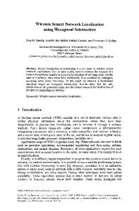
Fig. 1. A sequential discovery process. Black nodes are at known or previously estimated locations. Transmitting node 5 is localized using nodes 1, 2, 3 and 4.

1. INTRODUCTION Wireless sensor networks (WSNs) are commonly employed for the detection, localization and classification of events of interest for many military, research and commercial applications [1]. Common localization techniques include Time-ofArrival (TOA), Time Difference of Arrival (TDOA), Received Signal Strength (RSS) and Direction-of-Arrival (DOA) [1–3]. In all of these approaches, range or direction based parameters related to the location of a transmitting target of interest are extracted by observing the signal at a number of sensor sites at known locations. In this paper, a recently proposed wide aperture array localization algorithm [4] will be used to provide an initial coarse grained location estimate of transmitting sensor nodes at unknown locations for a network discovery algorithm. In contrast to conventional approaches, direction and range based information are jointly used to localize transmitting nodes by forming a large aperture array of nodes. This leads to improved localization accuracy [5]. Authors from Arizona State University are funded in part by the SenSIP Center. Authors from Imperial College are funded in part by the University Defence Research Centre (UDRC) in Signal Processing (MOD, UK). The authors were also supported in part by the British Council.

© EURASIP, 2012 - ISSN 2076-1465

A sequential discovery process is presented in this paper to locate a large number of sensor nodes. Considerable attention has been paid to the network discovery problem in the literature such as in [6–9]. In this paper, emphasis is placed on the actual localization approach employed which will fundamentally affect the performance of the discovery process. It is assumed that the actual discovery takes place in an ad-hoc manner. In particular, with reference to Figure 1, transmitting sensor nodes close to the anchors are first estimated, followed by those further away. Processing may take place in a distributed manner, involving only a selection of the nodes in the network. Hence, multiple transmitting nodes can be localized in different parts of the network at the same time. Additionally, many independent location estimates of a transmitting node may be obtained, which can then be combined using data fusion techniques [10, 11]. A drawback of sequential discovery arises when estimates of the sensor node locations contain uncertainties which will propagate through the network. This occurs because the localization algorithms assume that the sensors used in the localization procedure are at known locations. This makes early node local-

2278

izations markedly important and also stimulates the need for a fine grained localization procedure to improve the performance of the discovery process. Examples of potential finegrained localization approaches in the literature are presented in [12, 13]. However, we propose an array calibration technique which exploits the WSN as an array structure for fine grained node localization. This will be developed in future work. In this paper the following notation is used. A scalar is represented as x or X, a column vector is represented by x or X and a matrix is represented by X or X. Furthermore, (·) T H denotes a matrix transpose and (·) denotes the Hermitian transpose. In addition, X!Y and X"Y denote the Hadamard (element by element) product and division between the matrices X and Y respectively. Finally, R and C denote sets of real and complex numbers respectively. The remainder of this paper is structured as follows: In Section 2, the wide aperture array localization approach presented in [4] is summarized. Following this, in Section 3, the coarse component of the sequential network discovery algorithm is presented. In Section 4, simulation results demonstrating the effectiveness of this approach are given. Finally, in Section 5, conclusions and future work are presented. 2. LOCALIZATION USING WIDE APERTURE ARRAY PROCESSING Let N wireless sensor nodes with known locations form a sparse large aperture array. The Cartesian coordinates of the ith sensor node with respect to the array reference point is denoted by r i ∈ R3×1 . Assume the array operates in the presence of a single node transmitting a narrowband message signal m (t) with carrier frequency F c and is located at azimuth θ, elevation φ and range ρ 1 with respect to the array reference point (0, 0, 0). Without loss of generality the first node is located at r 1 = [0, 0, 0]T . The signal vector x (t) ∈ C N ×1 received by the array can be modeled as x(t) = q ! Sm(t) + n(t),

(1)

where the vector S represents the N -dimensional array manifold vector which describes the response of the array in the presence of the transmitting source and is a function of the array geometry, location of the transmitting node, and the carrier frequency. Furthermore, in equation (1), the vector q ∈ C N ×1 models the slow varying effects of the channel; and n (t) is the complex N -dimensional vector of the noise at the array elements, and is complex zero-mean additive white Gaussian noise 1 with power σn2 . Since the wireless array has a large aperture (i.e., far greater than a wavelength), the plane wave assumption will no longer be valid and hence a spherical 1 Note that if the noise is not white Gaussian, the received covariance matrix R should be factorized (for example via Cholesky factorization) and pre and post processed using the factorization before employing the proposed algorithm.

wave array response will be observed. Assuming omnidirectional sensor nodes ! $ # 2πFc " a −a S = ρ1 ·ρ !exp −j ρ1 · 1N − ρ ∈ C N ×1 , (2) c where a is a known constant scalar which represents the path loss exponent, c is the signal propagation speed and ρ is the vector of ranges from the source to each of the array elements: ρ = [ρ1 , ρ2,··· , ρN ]T ∈ RN ×1 .

(3)

Next consider L snapshots of data is received from the N sensor wide aperture array. The array signal received over this observation interval can be expressed as the matrix X ∈ C N ×L which follows the signal model in Equation 1 where, X = [x (t1 ) , x (t2 ) , · · · , x (tL )] .

(4)

Now consider that the array reference point is changed from the 1st to the ith sensor of the array. In this case, the new reference point is r i and the source is at range ρ i and direction (θi , φi ) relative to this new reference point. Thus, the measurements of x(t) are now taken with respect to r i . For the purposes of localization, this can be achieved for the matrix X by dividing the signals received at each sensor by the signals received at the i th sensor to form the matrix X i . Hence, Xi = X " (1N · rowi (X)) , i = 1, 2, · · · , N,

(5)

where rowi (X) denotes the ith row of the matrix X. The corresponding normalized covariance matrix is Ri =

1 N ×N Xi XH , i = 1, 2, · · · , N. i ∈ C L

(6)

It can be proved that the manifold vectors S i for i = 1, 2, 3, · · · , N , when the array reference point is at i th sensor in the array will be collinear to one another but have different complex magnitudes. This difference is exploited to estimate the location of the transmitter. Specifically, by rotating the reference point, constructing the received covariance matrix, and taking the average of the N − 1 smallest eigenvalues to form an estimate of the noise power in the channel, it is proved in [4] that the so-called signal eigenvalue λ can be extracted in each case by subtracting this estimate from the corresponding principal eigenvalue, γi = max (eig Ri ) , i = 1, 2, · · · , N,

λi = γi −

σ %n2 ,

i = 1, 2, · · · , N,

(7) (8)

where λi corresponds to the signal eigenvalue associated with the ith covariance matrix when the array reference point is at the ith array sensor. Using these eigenvalues, N − 1 metrics related to the ratio of ranges between the transmitting node and the array sensors can be constructed as ! $−2a λi ρi = , i = 2, · · · , N. (9) Ki = λ1 ρ1

2279

Initialization Step 1: Using the N anchor nodes as an array with known geometry r, estimate the location of a transmitting (i.e. i = (N + 1) th ) node over L snapshots using Equation (11). Step 2: Set i = N + 2; k = 1. Algorithm For the ith undiscovered node that transmits within a coverage range D, repeat the following steps until all the node locations have been estimated: Step 1: Find the number of nodes at known or estimated locations Nset within the coverage range. Step 2: If Nset ≥ 4 Then Form an array of the N set nodes with geometry r Else Move to Step 4. Step 3: Estimate the location of the transmitting node over L snapshots using Equation (11) and r. Step 4: i = i + 1; k = k + 1. Refinement Step 1: For the kth discovery iteration, set i = N + 1 and repeat the Algorithm using any node location estimates from previous iterations until k = K. Step 2: Combine the multiple estimates of the node locations using a fusion technique (e.g. take the average of the estimated locations).

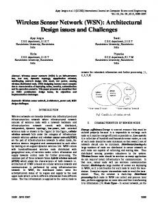
Fig. 2. Focussing vectors and loci used for localization in R 2 space. Fi respresents the ith focussing vector.

As shown in Figure 2, N − 1 circular loci can then be constructed using these metrics where the common point of intersection of these circles will correspond to the location estimate of the transmitting node. These loci will have centers rci ∈ R3×1 and radii Rci defined by r ci Rci

1 Ki2 = ri − r , i = 2, · · · , N, 2 1 − Ki 1 − Ki2 1 & & & Ki & & · %r1 − r i % , i = 2, · · · , N. = && 1 − Ki2 &

(10b)

Hr#m = b,

(11)

(10a)

In [5], Equations (10a) and (10b) have been extended to construct a set of linear equations:

where, in the general R 3 case, ' " # " #) H = 2 1N −1 r T1 − ( rT , 1N −1 − K2 ∈ R(N −1)×4 , b =

r #m with

=

(12) + * 2 2 2 2 (N −1)×1 %r1 % 1N −1 − ( rx − ( ry − ( rz ∈ R , (13) ' T 2 )T r m , ρ1 ∈ R4×1 , (14)

)T ' ( rx , ( ry , ( r z ∈ R3×(N −1) , r = [r2 , r3 , · · · , r N ] = (

Table 1. The proposed sequential discovery algorithm.

(15)

denoting the array sensor locations excluding the first sensor. In this paper, Equation (11) will be used for node localization. In [4], the upper bound on the RMSE of the localization approach is shown to depend on the number of array sensors N , input SNR, number of snapshots L, and the angle between

the focusing vectors. These focusing vectors point from each of the N − 1 locus centers to the location of the transmitting node (see Figure 2). As a result, the RMSE bound is determined by the array geometry as well as the location of the transmitting source. Hence, a good geometry to locate one transmitting source may not be good for another. To minimize the RMSE bound, #◦ angle between the N − 1 focusing " −1the . Note that when the angle between vectors should be N360 focusing vectors is 0 ◦ the loci become collinear and localization is not possible without ambiguity. Strategies should be developed to contend with such situations if the loci will be solved geometrically. The effect of the wide aperture array geometry on the performance of the array is discussed in terms of differential geometry in [14]. 3. THE SEQUENTIAL DISCOVERY ALGORITHM A coarse grained sequential network discovery process is presented which employs the wide aperture array localization process summarized in Section 2. The algorithm begins with N anchor nodes at known locations and M nodes at unknown locations. Each node has a coverage range of D. The order in which nodes are localized is arbitrary but it is intuitive that anchors are more likely to be within the limited coverage area of the closest transmitting nodes. Hence, closest nodes will be localized first. The effect of the localization order on the dis-

2280

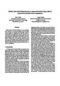
covery process performance is minimized by estimating each node location multiple times throughout the procedure. With reference to the algorithm presented in Table 1, for each transmitting node, K (a user selected parameter) independent estimates of the transmitting node location are attempted over time using an array made of all N set sensor nodes at known or estimated locations within its coverage area. Here, the minimum number of sensor nodes must be four in two-dimensional space. Nodes outside the coverage area are available for other uses in parallel. Hence, the distributed nature of the WSN can be exploited to make estimates of other transmitting nodes in other parts of the network simultaneously. In Step 2 of the Refinement, the K estimates of the transmitting source location are combined using a fusion technique (e.g. averaging). Using a more sophisticated fusion technique based upon the expected quality of the localization estimates computed as a function of, for example, the array geometry, may provide enhanced performance. If no array of at least four nodes can be constructed which lies within the coverage area of a transmitting node, the discovery process continues and localization of the node is attempted at a later stage when more nodes surrounding it have been localized. This takes place a maximum of K times before it is deemed that the node can not be localized. The proposed sequential discovery algorithm provides a robust localization procedure by producing multiple estimates of transmitting node locations, and revisiting nodes which cannot initially be localized. This is particularly important in a sequential discovery process to minimize the localization errors propagating to other nodes in the network. 4. SIMULATION RESULTS Consider a two-dimensional 500m×500m sensor field as shown in Figure 3. Assume N = 4 anchor nodes denoted by blue triangles are placed at known locations in the center of the field. These nodes are surrounded by two hundred sensor nodes denoted by green circles placed randomly at unknown locations following a uniform distribution. All nodes operate at a frequency of F c = 2.45GHz. In this example, the anchor nodes happen to land around the center of the map and are constrained to be close to one another (e.g. using a string) to allow the discovery process to initialize appropriately. Each node has a transmission range of D = 100m and the proposed coarse network discovery approach is applied under an SNR of 40dB using L = 100 snapshots per localization. A propagation constant of a = 4 exists in the simulation environment. Each transmitting node is estimated K = 10 times before the node is declared to be undiscovered. If multiple estimates are made then the average is taken. The final location estimates of the two hundred sensor nodes are shown in Figure 4 by red crosses. The average location error across all nodes is 0.9620m. It is clear that the location of nodes close to the anchors are estimated very accurately (i.e. node 5 has an error of 0.2mm). However, as expected, towards the edge

of the network, location uncertainties become significant due to the nature of the sequential discovery approach (i.e. node 203 has an error of 6.2218m). Furthermore, nodes 201 and 202 fail to be localized since there are an insufficient number of nodes in the transmission range for localization. It is important to note that at lower SNR×L the performance of the discovery process degrades rapidly as the location estimates of sensor nodes at the very core of the network become more degraded leading to even larger errors at the outer edges of the network. 5. CONCLUSIONS AND FUTURE WORK A wireless sensor network discovery algorithm was introduced in this paper which aims to estimate the location of a large number of wireless sensor nodes with a low coverage range in the presence of only a few anchor nodes at known locations. This was split into coarse and fine grained steps, and this paper proposed the use of a wide aperture array localization algorithm to implement the coarse localization step. Here, arrays of sensor nodes at known or previously estimated locations are constructed to estimate the location of transmitting nodes. Hence, the approach is sequential, implying that once the location of a node has been estimated, it can be used in the localization of other nodes. However, simulation results show that this leads to the propagation of node location uncertainties towards the edges of the network. This is due to the fact that the locations of the sensors used to localize these nodes are known with less certainty, but are assumed to be known perfectly. However, it can be shown that since the underlying localization procedure is more powerful than other localization algorithms in the literature (e.g. TOA, DOA, RSS, etc...), it will perform better in the discovery process than using any of these other techniques [5]. The proposed coarse network discovery procedure provides a good initial estimate of the node locations, particularly for nodes closest to the center of the network. It is clear that a procedure is needed to revisit the node location estimates and provide an enhancement. This is left for future work. Specifically, a fine grained network discovery phase will be developed using array shape calibration techniques. Other areas of interest lie in developing distributed algorithms to compute the covariance matrices for the wide aperture array processing technique, in order to reduce processing bottlenecks and to increase the speed of the algorithm. Furthermore, hardware validation of the overall network discovery algorithm is desirable. In [15], the wide aperture array localization procedure which forms the underlying localization algorithm in this paper is implemented using National Instruments USRP2 hardware [16] within an anechoic chamber. Furthermore, in [17], a Java-DSP software interface has been developed for communicating with wireless sensor nodes. This work provides a powerful platform to enable the testing and development of the proposed wireless sensor network discovery process in realistic practical environments.

2281

300 204

200

184

190 181

195 177

191

76

74

116

60

36

y (in meters)

69 106 108 92

71 67

73

155 167

144 152

186 188 192 194

1

46

82 89 130 114 102 153 131 112

35

81

-200

124

150

24

85

29

22

33 43

27

25

9193 110 128 135

104 121

117 127 129

77 87

62 66 79 98 88 70 113 86 95 132 123 143 111

50

163 156

118 154

122 134

169 172 201

174

149

0 x (in meters)

125

40

42 54

158 151 94

51 57 64

15

160

-100

20

61

78 84

119

189 180 175 176

137

7

39 47

101

173

170 182 99

196

168

48 52

12

23

30

56

63

161

105

83

49

2 365

9 13

115

199

-300 -300

16

37

100

17 19 10 11 8 4

197

187

28

26

21 18 14

68 139 145 138

-200

34

41 38 32

183

80

45

44 31

58

203

164

193 75

53

55

146

72

162 140

133 141

59

65

103 96

120 97

109 90

107

147

-100

126

136

159

0

157

178 171 166 148

142

179

100

185

165

200 198

202

100

200

300

Fig. 3. Sequential discovery with target nodes having a coverage of D = 100m with SNR = 30dB. Node locations are averaged over K = 10 localization attempts. Green circles represent actual node locations, blue triangles represent anchor nodes at known locations, and red crosses represent location estimates. All but nodes 201 and 202 are localized. Location uncertainties can be seen more predominantly at the edges of the network. 6. REFERENCES [1] Zhao and Guibas, Wireless Sensor Networks: An Information Processing Approach. Morgan Kaufmann Publishers, 2004.

[10] M. K. Banavar, C. Tepedelenlio˘glu, and A. Spanias, “Estimation over fading channels with limited feedback using distributed sensing,” IEEE Trans. Signal Processing, vol. 58, no. 1, pp. 414 –425, jan. 2010.

[2] J. Foutz, A. Spanias, and M. K. Banavar, Narrowband Direction of Arrival Estimation for Antenna Arrays. Morgan and Claypool Publishers, 2008.

[11] N. Kovvali, et al., “Least-squares based feature extraction and sensor fusion for explosive detection,” in ICASSP 2010, march 2010, pp. 2918 –2921.

[3] N. Patwari, et al., “Locating the nodes: Cooperative localization in wireless sensor networks,” IEEE SP Magazine, vol. 22, no. 4, pp. 54–59, June 2005.

[12] A. Savvides, C.-C. Han, and M. B. Srivastava, “Dynamic finegrained localization in ad-hoc networks of sensors,” in ACM MobiCom ’01, 2001, pp. 166–179.

[4] A. Manikas, Y. I. Kamil, and P. Karaminas, “Positioning in wireless sensor networks using array processing,” in IEEE GLOBECOM 2008, December 2008, pp. 1–5.

[13] J. Albowicz, A. Chen, and L. Zhang, “Recursive position estimation in sensor networks,” in International Conf. Network Protocols, nov. 2001, pp. 35 – 41.

[5] A. Manikas, Y. I. Kamil, and M. Willerton, “Source localization using large aperture sparse arrays,” IEEE Transactions on Signal Processing, 2012, to appear.

[14] G. Elissaios and A. Manikas, “Array formation in arrayed wireless sensor networks,” HERMIS-mu-pi International Journal (Mathematics and Informatics Science), 2005.

[6] H. Wymeersch, J. Lien, and M. Z. Win, “Cooperative localization in wireless networks,” Proceedings of the IEEE, vol. 97, pp. 427–450, February 2009.

[15] M. Willerton, D. C. Yates, V. Goverdovsky, and C. Papavassiliou, “Experimental characterisation of a large aperture array localisation technique using an SDR testbench,” SDRWInnComm, December 2011.

[7] C. Pedersen, T. Pederson, and B. H. Fleury, “A variational message passing algorithm for sensor self-localization in wireless networks,” ISIT, 2011. [8] M. Welling and J. J. Lim, “A distributed message passing algorithm for sensor localization,” In Proc. ICANN 07, 2007. [9] D. Moore, et al. , “Robust distributed network localization with noisy range measurements,” In Proc. SenSys 04, 2004.

[16] National Instruments, “NI universal software dio peripheral (USRP),” available online .

raat

[17] H. Kwon, et al., “Experiments with sensor motes and JavaDSP,” IEEE Transactions on Education, vol. 52, no. 2, pp. 257 –262, may 2009.

2282