Shape Decomposition and Understanding of Point Cloud Objects

Shape Decomposition and Understanding of Point Cloud Objects Based On Perceptual Information Xiaojuan Ning 1,2,∗

Er Li1,†

Xiaopeng Zhang1,‡

Yinghui Wang2,§

1

2

Department of Computer Science and Engineering, Xi’an University of Technology, Xi’an, China NLPR - LIAMA - Digital Content Technology Research Center, Institute of Automation, CAS, Beijing, China

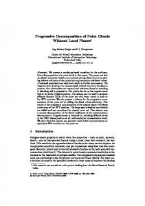
Figure 1: Overview of our algorithm. From a point cloud model, our algorithm extracts some perceptual feature points, according to which     the decomposition is implemented. Skeletal structure infers the topological information from the decomposed shape. Semantic graph shown   in the last column is generated with the assistance of decomposed shape and skeletons.              

Abstract

CR Categories: I.3.5 [Computer Graphics]: Computational Geometry and Object Modeling—Geometric algorithms, languages, and systems; I.4.6 [Image Processing and Computer Vision]: Segmentation—Region growing, partitioning;

Decomposition and segmentation of the objects represented by point cloud data become increasingly important for purposes like shape analysis and object recognition. In this paper, we propose a perception based approach to segment point cloud into distinct parts, and the decomposition is made possible of spatially close but geodetically distant parts. Curvature is a critical factor for shape representation, reflecting the convex and concave characteristics of an object, which is obtained by cubic surface fitting in our approach. To determine the number of patches, we calculate and select the critical feature points based on perception information to represent each patch. Taking the critical marker sets as a guide, each marker is spread to a meaningful region by curvature-based decomposition, and also further constraints are provided by the variation of normals. Then a skeleton extraction method is proposed and a labeldriven skeleton simplification process is implemented. Further, a semantic graph is constructed according to the decomposed model and the skeletal structure. We illustrate the framework and demonstrate our approach on point cloud data to evaluate its function to decompose object shape based on human perceptions. Meanwhile, the result of decomposition is demonstrated with extracted skeletons. Performance of this algorithm is exhibited with experimental results, which proves its robustness to noise.

Keywords: Shape Decomposition, Point Cloud, Skeletal Point, Semantic Graph, Perceptual Information

1

Introduction

Decomposing 3D objects into meaningful parts is a challenge but fundamental to shape understanding, shape information processing and shape analysis. The partition of a model into meaningful parts is referred to as shape segmentation or decomposition, which is an important area of ongoing research and remains an open research problem [Chen et al. 2009]. The decomposition results for 3D geometry have wide range applications in different branches of computer graphics and computer vision, including computer animation, modeling, shape analysis, classification, object recognition and 3D model retrieval [Shlafman et al. 2002], [Katz and Tal 2003], [Funkhouser et al. 2004]. One of the most popular representations for 3D shape is mesh model. Most proposed segmentation methods take mesh model as input, and rely on topological information of the model, i.e., edges and faces. However, due to the difficulties of processing and manipulating large mesh connectivity information, many researchers question the future utility of polygons as the fundamental graphics primitive [Gross and Pfister 2007]. On the other hand, with the development of modern 3D scanning systems, another representation – raw point cloud data emerged, which can be used to acquire both geometry and appearance of complex, real-world objects. However, point cloud data, which only includes raw data point coordinates, can not be processed by the existent mesh segmentation algorithm (most mesh segmentation algorithms can not be applied directly).

∗ e-mail:[email protected] † e-mail:[email protected] ‡ e-mail:[email protected] § e-mail:[email protected]

Copyright © 2010 by the Association for Computing Machinery, Inc. Permission to make digital or hard copies of part or all of this work for personal or classroom use is granted without fee provided that copies are not made or distributed for commercial advantage and that copies bear this notice and the full citation on the first page. Copyrights for components of this work owned by others than ACM must be honored. Abstracting with credit is permitted. To copy otherwise, to republish, to post on servers, or to redistribute to lists, requires prior specific permission and/or a fee. Request permissions from Permissions Dept, ACM Inc., fax +1 (212) 869-0481 or e-mail [email protected]. VRCAI 2010, Seoul, South Korea, December 12 – 13, 2010. © 2010 ACM 978-1-4503-0459-7/10/0012 $10.00

In this paper, our work focus on the decomposition and understanding of point cloud data. We may require shape decomposition or segmentation to lead us a way to understand the shapes. The decomposition is mainly based on human visual perception, which is

199

 

referred to as the basic capability of the human visual system to derive relevant groupings and structures from 3D objects without prior knowledge of its contents.

into super-nodes. The second phase is hierarchical segmentation which bisects the set of super-nodes while ensuring that similar super-nodes remain together. Then in the last stage it refined the segmentation to ensure that all segments contain at least one significant feature. The method is effective to capture geometric features in complex point sets. However, one of the disadvantages is the computation time especially on the geodesic distance.

Our contributions of the paper are in five aspects. First, we present a framework for shape decomposition with several steps including perceptual feature points selection, curvature-based decompositions and etc. Second, we present a new method for critical feature points extraction based on contour points and clustering, which can be implemented automatically. Third, a skeleton extraction algorithm is proposed based on the decomposition, and a label-driven skeleton simplification process is presented to make more robust shape skeleton. Fourth, a semantic graph is constructed from the decomposed shape and skeletal structure. Finally, we analyze the performance of our algorithm. The complete overview of our algorithm is shown in Figure 1.

Based on the work in [Yamazaki et al. 2006], Zou et al. [Zou and Ye 2007] proposed a hierarchical point cloud segmentation algorithm based on multi-resolution represent of point cloud. This approach constructed a simplified geometry by its BVH (Boundary Volume Hierarchy). Then a fuzzy clustering segmentation algorithm is implemented. Although this method can process large scale point cloud rapidly, it also leads to coarse boundary. Reniers and Telea [Reniers and Telea 2007] presented a framework for segmenting 3D shapes into meaningful components using the curve skeleton. This method is based on voxel-shapes, which can not be applied to point cloud data.

The outline of this paper is as follows. We briefly discuss respectively the state-of-the-art segmentation method on the point cloud data in section 2. Overview of our algorithm is illustrated in section 3. We then proceed with the implementation details of point cloud shape decomposition in Section 4. Further skeleton extraction and simplification are illustrated in section 5 and a semantic graph is constructed to describe the shape. Experimental results are illustrated, and we analyze the results of our approach as well in Section 6. Based on the experiments, conclusions end Section 7.

2

Richtsfeld [Richtsfeld and Vincze 2009] segmented 3D object from point cloud data in a hierarchical manner, which is based on radial reflection. The method begins from core extraction by computing smallest enclosing sphere of points. And after the core part is found, all other segments of the point cloud are extracted by floodfilling. Meanwhile, the segmentation results is improved by the normal vector. In addition, they have considered pose-invariant model by generating a 3D mesh with power crust algorithm. The method is only useful for the data which have core parts. Also the method in [Ma et al. 2007] is effective in segmenting point cloud, but it shows disadvantages in high complexity of the algorithm.

Related Work

There has been a considerable research work relevant to 3D object segmentation, most of which require that a surface model is provided explicitly via a triangle mesh [Yamauchi et al. 2005], [Liu and Zhang 2004], [Page et al. 2003] or converting point cloud data into a mesh [Joachim et al. 2003].

All the methods aforementioned all paid attentions to how to decompose the objects in point clouds, and they did not make further work to understand and describe the shape. In this paper, we propose a SDAU (Shape Decomposition And Understanding) framework based on human perception, which is to aggregate the points with similar attributes and construct the semantic graph of 3D objects to make more explicit shape information. For the decomposition we proposed a boundary-based feature point extraction method, with curvature-based and variation of normal vector constraints to decompose 3D objects into parts. The skeleton extraction process is also implemented to represent the topological information of shape.

Based on different aims, segmentation methods can generally be classified into two types: part-type segmentation and patch-type segmentation [Shamir 2004]. Part-type segmentation tries to segment models into visually meaningful parts to human beings, and patch-type segmentation must be topologically equivalent to a disk, so as to not impose large distortion after parametrization onto 2D. In addition, segmentation methods can be roughly categorized into three types: Edge-based, region-based and hybrid segmentation methods [Liu and Xiong 2008]. Edge-based methods attempt to detect the discontinuities in the surface that form the closed boundaries of different segments. Two approaches are classified as bottom-up and top-down for region-based method. Top-down methods start by assigning all the points to one group and fitting a surface to it. For bottom-up approaches, a number of seed regions or a seed point are chosen first, and then grow by adding neighbor points based on some compatibility thresholds. The hybrid methods have been developed using the edge-based and region-based information.

3

Algorithm Overview

This section begins with a few notations and some terms with its corresponding symbols in this paper. Then we outline our shape decomposition and understanding framework (short for SDAU framework). Shape Decomposition can be described as follows: for a shape S represented by point cloud, divide it into Sm parts (m is not less than the number of critical points), i.e. S = m i=1 Si , Si ∩ Sj = ∅. Here a Si is called a patch of S.

Recent advances in point cloud segmentation are typically Joachim et al. [Joachim et al. 2003], Yamazaki et al. [Yamazaki et al. 2006], zou et al. [Zou and Ye 2007] and Richtsfeld [Richtsfeld and Vincze 2009]. Joachim et al. [Joachim et al. 2003] have done some pioneer research on point cloud segmentation. They propose a mathematic definition of features and translate it to discrete domain. After that they improve their method to segment and match the noisy point cloud, but it still requires delaunay triangulation of the noisy point sample.

Critical Feature Point Set. For every point pi ∈ P, let Scp be the contour points set and Hp be the convex hull of the set Scp . Then the critical point determined by the clustering of Hp is denoted by M Sp = {M1 , M2 , ..., Mm }. Convexity Representation. Curvature Cp for each point pi , and the variance Vkp of normal is another way to weigh the convexity and concavity of shape S.

Yamazaki et al. [Yamazaki et al. 2006] proposed a three-phase process to segment point sets. The first phase is feature identification which performs hierarchical segmentation by coarsening the input

Decomposed Skeleton. The decomposed skeleton is represented by DS1 , DS2 , ..., DSm for corresponding decomposition patch

200

SDAU Framework

Input

Normal and Curvature Estimation

Label Initialization

Contour Points

Constrain Condition

Convex Hull

Semantic Graph

Decomposition  

Shape Clustering

Marker Set Simplification Skeleton

Smooth, Centrality

 

Initial Skeleton

 

Skeletal Point Figure 2: Diagram of Our Framework.

S1 , S2 , ..., Sm .

4

Semantic Graph. Represented by G =< V, E >, it is used to describe the topological relations of the shape. V = {V1 , V2 , ..., Vm } denotes each part in decomposed shape and E is the connection between each two parts.

4.1

Shape decomposition K Nearest Neighborhood Graph

Finding neighboring points for one given point is a crucial step in our algorithm. And K-NN (k nearest neighbors) graph is used, which means that k neighboring points for point p are selected from the point cloud data P = {pi }i=1,2,...,n which have the minimum Euclidean distance. In fact the distances between p and each point in the whole data are calculated and sorted ascending, and then the first k points are chosen as the k neighboring points (i.e. k nearest neighbor graphs are able to connect regions on different scales, since only the absolute neighborhood ranking is of interest). The number of k is determined according to the point density, and it can avoid degenerated cases that a point has no neighboring points. In our approach, searching for the neighboring points is achieved by kd tree algorithm in order to organize the data. We have adopted the ANN library (Approximate Nearest Neighbor) which supports data structures and algorithms for both extract and approximate nearest neighbor searching in arbitrarily high dimensions.

Figure 1 provides an example to describe the shape decomposition and understanding framework for point cloud data. The proposed decomposition method is based on the curvature and variation of normal vector which can be concluded from the first column to the fourth column in Figure 1. The whole process for the decomposition and understanding of point cloud can be summarized in Figure 2. There are three steps in decomposition stage: detecting the boundary of the raw data using alpha shape to make it easier to locate the feature points; finding the inflexion (convex and concave points) in the boundary; finally, using region growing to obtain the optimal segmentation results. The pipeline of decomposition can be illustrated as follows. At first, the algorithm calculates the normal vector Np and curvature Cp for each point p. Then the contour points set Scp and convex hull Hp of Scp are determined which will be used to find the feature points representing distinct feature of the point model, and meanwhile the clustering of the points in Hp is implemented to get the unique critical points set Sp (the user can also intervene to provide guidance). Based on the feature points (accord with human perception), our algorithm automatically segments the point cloud into a set of meaningful sub-parts by region growing based on minimal rule and a constrained condition rely on the variation of normals.

4.2

Concave and Convex Representation

As well as normal, normal curvature, principal direction and Gauss curvature, curvature is one of the effective features for surface which can be used as local differential geometry measurement. Curvature plays an important role in object segmentation, since concave point and convex points are feature points of objects which could be estimated by curvature. There are various methods for estimating higher order information such as curvature from discrete surface information. In our paper, the curvature of each point p is estimated by cubic surface fitting, which will be used as a criterion for region growing in segmentation process. Each point p in the point cloud can be characterized by the Darboux frame at p, i.e.

Based on decomposition results, the skeletal points are extracted and simplified, and also the semantic graph is generated. We can see from the last three pictures in Figure 1.

∆p = (p, n, e1 , e2 , k1 , k2 ),

201

(1)

(a)

(b)

(c)

(d) (a)

Figure 3: Contour Points Calculation.

Figure 4: Optimal Critical Points. (a) Points of Convex Hull (b) Critical Points.

where n is the surface normal vector at p, and e1 , e2 are the principal directions corresponding to the principle curvatures k1 , k2 (k1 ik2 ) respectively.

critical points selection.

v The unit normal vector n is given by n = ||rruu ×r , r(u, v) is a lo×rv || cal parametrization of a surface in the neighborhood of p. The maximum and minimum principal curvatures k1 and k2 can be computed by the Weingarten curvature matrix.

For each point in Hp , cluster together its k nearest neighboring points within a given distance constrain Dth which is determined by the minimum distance multiplied by a multiplier. According to each labeled cluster, those clusters whose points number is less than a given threshold are filtered. Then in the remaining clusters from each of which we select one point, and then final marker sets M SP are finally determined. Nevertheless, due to the weakness of the k-nearest neighboring, some feature points can not be detected accurately. In such cases, the user can intervene to provide further guidance to obtain appropriate feature points which must satisfy human perception.

Let λ1 and λ2 (λ1 ≥ λ2 ) be the eigenvalues of Weingarten matrix W, and v1 , v2 are the corresponding eigenvectors, then k1 = λ1 , k2 = λ2 . The Gaussian curvature K and mean curvature H are defined as K = k1 k2 , H = (k1 + k2 )/2. In our paper, the Gaussian curvature K is a criterion to weigh whether the points reside on convex or concave parts. Generally, the convex parts may have positive maximum curvature, and the concave parts would have negative minima curvature.

4.3 4.3.1

4.4

Contour Points and Feature Points Determination

4.4.1

Contour points of 3D objects from point cloud data can be determined by projecting the original points into its representative plane, and then a boundary detection algorithm is used to extract accurate set of contour points Scp = {Cp1 , Cp2 , ..., Cpr }.

Vkp =

kp =

Mλ0 (Mλ0 ≤ Mλ1 ≤ Mλ2 ) Mλ0 + Mλ1 + Mλ2

(3)

(4)

i=1

If the point is on a smooth surface then the variance Vkp is very small (almost 0). The distribution of kp for different data are distinct and we show several experimental results for some selected data. It is useful for further threshold selection and also has effect on the segmentation results.

The convex hull Hp of a set of points P in n dimensions is the intersection of all convex sets containing all points set P . For N points p1 , p2 , ..., pn , the convex hull Hp is then given by the smallest convex set that contains P . Generally, the local curvature maxima is the convex points. This process aims at finding the critical points robustly. For those points Cpi in Scp , a set of points Hp reside on the outer convex hull is automatically calculated.

k S

n 1X (kpi − k)2 n i=1

where Mλ0 , Mλ1 and Mλ2 are the eigenvalues of the covariance N P matrix M , and M = (pi − p¯)(pi − p¯)T .

Optimal Critical Feature Points

Where Scp =

Constraints Condition

The variance in the normal direction over the variance in the neighborhood is used to weigh whether the region is smooth or not, which can be represented as follows.

Let p be one point in original point cloud P , search for all its k (k = 10 ∼ 30) neighboring points (within distance 2r) set Q = q1 , q2 , ..., qk . Select any point qi from Q, and we can compute a circle center C according to the two points p, qi and a radius r (defined by user, for most of the data r = 1.0). In general, if point p is a contour point then all its neighboring points are not within the circle, i.e. the distance to C is larger than r. We can obtain the contour points from original point cloud data, the process is shown in Figure 3.

Hp = ConvexHull(Scp )

Region Decomposition Process

The Minima Rule is a theory that defines a framework for human perception that might decompose an object into its constituent parts, which has already been presented for segmentation of CAD models and meshes [Page et al. 2003]. The rule provides boundaries along lines of negative minima curvature.

Contour Points

Further critical points are determined by the local curvature maximum which is often located on the boundary or contour, so it is more essential to obtain the contour points.

4.3.2

(b)

4.4.2

Region Growing

If the critical points are found, we can continue the decomposition of point cloud. Here, our method is used to identify connected point sets by growing the seed points using nearest neighboring clustering. The process is based on the minima rule and the constrains that the points belong to one patch may have little variation of normal vectors. Different parts will be disconnected at the mutation of the local curvature. The algorithm is based on the following steps:

(2)

Cpi . Hp , contains less points than Scp and pos-

i=1

sesses the local maxima characteristics, which is helpful for further

202

S2 

S1 

S1 

(a)

(b)

S2 

S1 

S3 

S3 

S2  S3 

(a)

(b)

(c)

(d)

(c)

Figure 5: Segmentation of Teapot Data. (a) Teapot Data (b) Feature Points (c) Segmentation Results.

• Input point cloud data P and the corresponding feature points set M Sp .

Figure 6: Illustration of Decomposed Skeleton. (a) Decomposed shape S1 , S2 , S3 . (b) Shortest path connecting each critical point of Si with the center point. (c) Detect the variation of the point label. (d) Simplified skeleton.

• Compute the curvature sets Cp , normal sets np for each point in P , and the variance of normals kp . • Define three critical threshold kth (variance of normals), distance threshold Dth and k neighborhood number N .

(2) After determining the core point O of the object, we use Dijkstra’s shortest path algorithm to compute the distance between  two points. Then connect each critical point Ci with O by the shortest path which can be considered as the initial skeleton IS = {IS1 , IS2 , ..., ISk } consisted by surface points ;

• Search the k nearest neighboring points for each pi in M Sp , namely Nnp . • Sort the points in Nnp in the light of its curvature, and start region growing from the point with maximum curvature.

(3) Taking the initial skeleton as input, we use a repulsive force to push each point in IS into the interior of the object. Thus the final skeleton is generated;

• The seed point and its neighboring points within Dth are belong to one patch if vkp of points in Nnp are less than kth . If the point is unlabeled and its corresponding kp is less than kth , then it will belong to the same region with seed point.

(4) To make the skeleton more robust and to ensure that points on the skeletal structure can provide a smooth connection between the initial skeletal points, a simple smoothing strategy is implemented. Start from the core point of the model vmin , if the angle between vi vi+1 and vi+1 vi+2 is larger than a threshold ε then we will sub0 stitute vi+1 with vi+1 = (vi + vi+2 )/2.

• On the conditions that the seed points and all its neighborhood are labeled, but not all the points are labeled, then we require to select another one with maximum curvature from the remaining points in order to further region growing. The point clouds are segmented into different components based on these steps. Figure 5 displays the decomposition process of teapot.

The repulsive force [Wu et al. 2003] can be calculated by WF (x) =

5

Decomposition based Skeleton Extraction

F (||qi − x||2 ) · (qi − x)

Where F (r) = r−2 , which represents the Newtonian potential function. V (x) = {q1 , q2 , ..., qk } is the k nearest neighboring point set. Then we can assign the initial position by pushing pi (a point in the initial skeleton) into the interior of the object toward the reverse surface normal direction, then apply the shrinking procedure: pi+1 = pi + normalize(WF (pi )) ∗ e (8) where e is the distance defined by user. The iteration stops until |WF (pi+1 )| > |WF (pi )|

Skeletonization Algorithm

and the final position of pi is recorded.

Our shape decomposition gives rise to a novel skeleton extraction algorithm which can be summarized as follows:

 

(1) We construct a discrete function f that measures the centrality of a point with the surface, which is defined as the average geodesic distance. X 2 f= G (p, pi ) (5)

 

p∈P

Here the core point O of the whole model is defined as the point with the minimum average geodesic distance. vmin = argmin(f )

(7)

qi ∈V (x)

Skeletons are beneficial for various applications, including matching, retrieval, metamorphosis and computer animation [Katz and Tal 2003]. Previous algorithms are based on medial surface extraction, level set diagrams or Reeb Graphs. The Morse theory was originally developed to study the relationship between the shape of a space and the critical points of smooth functions defined on the space [Milnor 1963]. Recently, it has been applied in skeleton extraction [Wu et al. 2003], inspired by which we propose a skeleton extraction algorithm based on the shape decomposition results.

5.1

X

Figure 7: Semantic Graph Generation.

(6)

203

(9)

 

(a)

(b)

(c)

(d)

(e)

Figure 8: Decomposition process of Table.

5.2

Label-driven Skeleton Simplification

sume that all the node is given according to the decomposed results, and then we start from VO to determine the connection relationship based on the path that skeletal points pass through. It is easier to draw a clear semantic graph of each shape, according to which the following work can be further implemented, e.g. shape-based 3D retrieval, shape semantic analysis and etc.

Let S1 , S2 , S3 , ..., Sk be the k segmentation of model S, where segment Si = {v1 , v2 , ..., vm } which may contain m points or vertex. Figure 6(a) shows a decomposed shape which contains three subparts S1 , S2 , and S3 . For each segment Si , there is a critical point Ci . In Figure 6(b), two black points C1 and C3 are the critical points corresponding to S1 and S3 , and the red points O is the central points.

6

We now investigate the behavior of the algorithm through point cloud data. Algorithms are programmed with VC++ and OpenGL for rendering. All experiments are implemented on a PC with R IN T EL CoreT M 2 CPU, and 2G memory.

The path connecting Ci and O could be labeled according to the decomposition results (see in Figure 6(b)). Then a label-driven algorithm is proposed to simplify the smooth skeleton. The joints of two different parts are calculated directly from the structure of decomposition since the label variance make it clear to distinguish each other (see in Figure 6(c)). The simplified skeleton are composed by directly connecting the critical points with the central points (see in Figure 6(d)). It is essential that skeleton which depends on the position of critical points and central points must reside on the central position in the shape model. A simple way to achieve this is to guarantee that there are transition points between central points and all other critical points.

To begin, the marker set M SP is constructed from point cloud data P . Markers in M SP are acquired based on the contour points and curvature extremum.

6.1

Data Set

In this paper, we employed data download from “AIM@SHAPE” web site (http://shapes.aim-at-shape.net), and some data are from the Princeton Segmentation Benchmark [Chen et al. 2009] which provides 19 categories of meshes. Our method are evaluated on several typical data sets to demonstrate the robustness of our method, we first collect the point data and then progressively add some random Gaussian noise to simulate the irregular data.

This algorithm is general, fully automatic, simple and fast. It is thus beneficial for applications requiring automation as well as for novice users of applications where user-intervention is acceptable or desirable. Figure 10 demonstrates the extraction and simplification of skeletons for static horse object.

5.3

Experiments Evaluation and Discussion

Shape Understanding and Analysis

6.2

The skeleton of a shape could provide an intuitive and effective abstraction which facilitates shape understanding and manipulations. In this section, we exploit the Semantic Graph by the decomposed shape and skeleton structure. Semantic Graph, as a representation of shape, can also describe the topology of objects more efficiently and has wide applications in 3D model retrieval. The semantic graph is unique and could capture the critical topology information of the object.

Feature Points Selection

The critical points for point cloud data are determined by contour points (see in Figure 8(b)). We should select several feature points which meet human perception, so we obtain the points on the convex hull (see in Figure 8(c)) and then refine them by further clustering (i.e. k-nearest neighborhood clustering). The results are shown in Figure 8(c) and Figure 8(d). The points in blue color in Figure 8(d) is the refined convex hull, and other points in different colors represented different clusters. According to the clustering results we choose one points from each cluster which will be considered as a seed point for further region growing.

Semantic Graph in our paper can be defined as G =< V, E >, where V = {V1 , V2 , ..., Vm }, Vi is a node representing the decomposed subparts Si , E = {E1 , E2 , ..., Em−1 }, Ei is the topology relationship between two subparts if there is a joint that transited from one labeled parts to another when connecting the skeleton points. Then after decomposition, we regard each part as a node ( represented by the left one in Figure 7) and two nodes have an edge if and only if they are adjacent. The adjacent relations can be evaluated by the skeletal structure (the middle one in Figure7).

6.3

Decomposition Results

In this section, we demonstrate the results of decomposition from regular point cloud data and data with noisy points. Decomposition on Regular Point Cloud Data

We have obtained the central points O in Eq.6 with minimum geodesic distance. It will be the core point VO of semantic graph if the part it belongs to is the largest one in original point cloud. As-

The decomposition results on regular point cloud data are displayed in Figure 8, of which the selection of feature points are all based on human perception.

204

Table 1: Data Sets and Results Analysis. kNN: k-nearest neighbor; Bou: boundary detection; Clu: clustering for further critical points selection; Cri: final critical points determination; Seg: segmentation process. Here n is the original points number, Cp is the number of contour points, Ms is the number of final marker set.

Dataset Ant Table Palm Tippy Horse Teapot

Data Size n 8176 13579 11413 9548 8078 6678

Contour Points Cp 428 562 332 556 356 184

Marker Set Ms 9 4 6 8 8 4

kNN 0.015 0.047 0.02 0.01 0.015 0.016

Run time(sec) Bou Clu 3.594 0.031 6.1 0.06 5.0 0.31 4.2 0.07 3.906 0.025 3.328 0.063

Cri 0.016 0.015 0.032 0.01 0.016 0.001

Seg 4.609 12.172 7.625 6.840 4.750 3.437

• Boundary detection: O(n log(n)); • Clustering for final critical:O(n log(n)); • Critical points determination: O(log(n)); (a)

(b)

• Segmentation: O(n2 log(n)).

(c)

In addition, Table 1 demonstrates the experimental data and the algorithms running time, which shows good performance for several objects. Compared with other methods, our method performs well both on the running time and computational complexities.

(d)

(e)

(f)

Figure 9: Decomposition results on Noisy Data. (a),(b),(d),(e) is respectively the teapot model and palm model after adding gaussian noise (c) and (f) is the decomposition results. (a)

(b)

(c)

(d)

In Figure 8, we show the segmentation process of table data, the critical points (Figure 8(d)) are obtained by convex hull (Figure 8(c)) and contour points (Figure 8(b)). According to the critical points, table data is segmented into 4 regions in Figure 8(e) which satisfies human perception. Decomposition on Data with Noises Missing data and noisy points are common during 3D shape acquisition. In this section, to demonstrate the robustness to noisy points, we collect some data by adding noisy points such as Figure 9(a) and Figure 9(d). For the teapot model, we have added 0.1% gaussian noise and 1% gaussian noise for palm model.

Figure 10: Skeleton Extraction. (a) Initial surface point skeleton (b)Central skeleton (c) Smooth skeleton (d) Simplified skeleton.

In Figure 9, we show the decomposition results on the data point with noise. Figure 9(a) and Figure 9(b) is the teapot model after adding noise, Figure 9(a) shows the point distribution and Figure 9(b) demonstrates the mesh distribution. Figure 9(d) and Figure 9(e) also show noisy palm model. The results from Figure 9(c) and Figure 9(f) suggest the potential applicability of our method to the decomposition of irregular data when there is much more noise. There is no need to denoise the raw data. We can conclude that our method is effective and is robust to noise.

6.4

Skeletonization

Figure 10 demonstrate some decomposed shape skeleton. Most of the obtained parts seem meaningful. We derive the skeletal hierarchy and the joint positions automatically and, in may cases, the skeletons actually resemble the real-world skeletal structure of these shapes. The results also show that the skeleton of the object can be a better shape descriptor, and the shape decomposition lays solid foundation for the extraction and simplification of skeleton.

On the whole, our method is effective, practical and easy to implement. The computational complexities of the different steps are illustrated as follows:

Skeletonization times encompass both the initial skeletonization, smoothing the skeleton and simplification process. Skeletonization times were trivial in all examples and almost all under 0.01 seconds.

• k-nearest neighboring computation: O(kn log(n));

205

6.5

Limitations

J OACHIM , T. D., G IESEN , J., AND G OSWAMI , S. 2003. Shape segmentation and matching with flow discretization. In In Proc. Workshop on Algorithms and Data Structures, 25–36.

Our decomposition framework is designed for objects represented by point cloud data. Our algorithm requires the detection of critical points which is based on projected 2D information. It is applicable for diverse data, and for few data it needs some user queries to select feature points due to inappropriate projection. In addition, although our decomposition results are better than other algorithm for point cloud data, there are still limitations that it is still a challenge to determine the smooth boundary for some complex data. In addition, our method can not deal with incomplete point clouds, e.g. unilateral scanned data or large missing data, which will become as the further research.

7

K ATZ , S., AND TAL , A. 2003. Hierarchical mesh decomposition using fuzzy clustering and cuts. In SIGGRAPH ’03: ACM SIGGRAPH 2003 Papers, ACM, New York, NY, USA, 954–961. L IU , Y., AND X IONG , Y. 2008. Automatic segmentation of unorganized noisy point clouds based on the gaussian map. Comput. Aided Des. 40, 5, 576–594. L IU , R., AND Z HANG , H. 2004. Segmentation of 3d meshes through spectral clustering. In PG ’04: Proceedings of the Computer Graphics and Applications, 12th Pacific Conference, IEEE Computer Society, Washington, DC, USA, 298–305.

Conclusions and Future Work

M A , Y., W ORRALL , S., AND KONDOZ , A. M., 2007. 3d point segmentation with critical point and fuzzy clustering.

In this work, an algorithm is proposed for decomposing a point cloud model, representing an arbitrarily shaped object, into meaningful components. Our method works on the point set directly without triangulation or other preprocessing. The key steps in this work are critical points identification and segmentation. The selection of critical points is based on the human perception and an assumption that those points with local curvature maxima are almost reside on the convex surface. Based on this, we proposed to obtain them by several steps: contour points calculation (Scp set), convex hull for further constrains of Cp , clustering of the remaining points in Hp , and then final critical points are generated. Based on the critical points, the decomposition process continues with the constrains that points belonging to one smooth surface may have smaller variation of curvatures. Based on shape decomposition, a novel skeleton extraction algorithm is implemented to obtain the decomposed skeleton, and then the skeleton is refined to simplify it by a label-driven method. The semantic graph of 3D object can be obtained from the decomposition results and the skeletal structure. Experiments demonstrate the robustness and effectiveness of the proposed decomposition method, which has been tested on different 3D models and has obtained good results from most of them. Also the extracted skeleton and semantic graph of 3D object is very useful in different applications.

M ILNOR , J. W. 1963. Morse theory. Princeton University Press. PAGE , D. L., KOSCHAN , A. F., AND A BIDI , M. A. 2003. Perception-based 3d triangle mesh segmentation using fast marching watersheds. In in Proceedings of the International Conference on Computer Vision and Pattern Recognition, II, 27– 32. R ENIERS , D., AND T ELEA , A. 2007. Skeleton-based hierarchical shape segmentation. In SMI ’07: Proceedings of the IEEE International Conference on Shape Modeling and Applications 2007, IEEE Computer Society, Washington, DC, USA, 179–188. R ICHTSFELD , M., AND V INCZE , M. 2009. Point cloud segmentation based on radial reflection. In Computer Analysis of Images and Patterns, Springer-Verlag, Berlin, Heidelberg, 955–962. S HAMIR , A. 2004. A formulation of boundary mesh segmentation. In 3DPVT ’04: Proceedings of the 3D Data Processing, Visualization, and Transmission, 2nd International Symposium, IEEE Computer Society, Washington, DC, USA, 82–89. S HLAFMAN , S., TAL , A., AND K ATZ , S. 2002. Metamorphosis of polyhedral surfaces using decomposition. In Computer Graphics Forum, 219–228.

Future work will concentrate on how to improve the boundary between clusters, since for some data the boundary between two different patches is not sufficiently smooth.

W U , F., M A , W., L IOU , P., L AING , R., AND O UHYOUNG , M. 2003. Skeleton extraction of 3d objects with visible repulsive force. In Eurographics Symposium on Geometry Processing. YAMAUCHI , H., L EE , S., L EE , Y., O HTAKE , Y., B ELYAEV, A., AND S EIDEL , H.-P. 2005. Feature sensitive mesh segmentation with mean shift. In SMI ’05: Proceedings of the International Conference on Shape Modeling and Applications 2005, IEEE Computer Society, Washington, DC, USA, 238—245.

Acknowledgment This work is supported in part by National Natural Science Foundation of China under Grant No. 60970093, 61072151, 60902078 and 60872120; and in part by the National High Technology Development 863 Program of China under Grant No. 2008AA01Z301.

YAMAZAKI , I., NATARAJAN , V., BAI , Z., AND H AMANN , B. 2006. Segmenting point sets. Shape Modeling and Applications, International Conference on 0, 6.

References

Z OU , W., AND Y E , X. 2007. Multi-resolution hierarchical point cloud segmenting. In IMSCCS ’07: Proceedings of the Second International Multi-Symposiums on Computer and Computational Sciences, IEEE Computer Society, Washington, DC, USA, 137–143.

C HEN , X., G OLOVINSKIY, A., , AND F UNKHOUSER , T. 2009. A benchmark for 3D mesh segmentation. ACM Transactions on Graphics (Proc. SIGGRAPH) 28, 3 (Aug.). F UNKHOUSER , T., K AZHDAN , M., S HILANE , P., M IN , P., K IEFER , W., TAL , A., RUSINKIEWICZ , S., AND D OBKIN , D. 2004. Modeling by example. ACM Trans. Graph. 23, 3, 652– 663. G ROSS , M., AND P FISTER , H. 2007. Point-Based Graphics. Morgan Kaufmann publisher.

206