Conventionally, the optimal shape design problem consists of minimizing an .... applied to the domain of the unit cell Ω (in our case, a periodic distribution of fibers is ..... In both cases of volume ratios we used the following material properties of.
Computer Aided Optimum Design in Engineering X
57
Shape optimization of composites based on minimum potential energy P. Procházka Czech Technical University in Prague, Czech Republic
Abstract Shape optimization of fibers based on the highest bearing capacity of composite aggregate on a unit cell is studied using Inverse variational principles. They have been applied mostly in connection with finite elements. It appears now that boundary elements are much more efficient. On the other hand, it is necessary to find an appropriate function, which describes boundary density of potential energy and at the same time variational bounds or homogenization of the composite have to be carried out. If one starts with homogenization, a mathematical formulation has to prove that a solution exists and is unique. The latter problem seems not to be as simple as it first seems. Additional constraints must be introduced to ensure the uniqueness of the solution. If bounds are sought, we start with extended Hashin–Shtrikman principles. A study is carried out for different relations of fibers and matrices. Keynotes: optimization, Inverse variational principles, classical composites.
1
Introduction
Conventionally, the optimal shape design problem consists of minimizing an appropriate cost functional with certain constraints, such as equilibrium and compatibility conditions and design requirements. The formulation of the cost function depends on the concrete intention of a designer. One of a reasonable and practical form of the cost function concerns the minimization of the strain energy of the body subjected to a specific load. Such a problem can easily be formulated in terms of inverse variational principles, which assure that the surface energy attains its minimum. The inverse variational principles are naturally connected with the finite element method, which starts with energetical formulation. But, the FEM is less WIT Transactions on The Built Environment, Vol 91, © 2007 WIT Press www.witpress.com, ISSN 1743-3509 (on-line) doi:10.2495/OP070061
58 Computer Aided Optimum Design in Engineering X suitable for the problems involving the optimal shape of boundary because of the division (in any case compulsory when using the FEM) of the domain, while the boundary element method seems to be more suitable for such problems as it does not require domain meshing. On the other hand, the direct connection of the BEM with the variational principles is not seen at first sight and desires a deeper study. Inverse variational principles, leading to the optimization of surface energy of bodies, were established by Prof. Bufler from Darmstadt University, Germany, at the end of the 1960s. Later on, they were developed by some authors, but published mostly at local, although including some international, conferences. An interesting application of the inverse variational principles is issued in [1, 2], where numerical experience is discussed. The results from these discussions are used in our paper. Numerical tools for solving the problems in terms of the inverse variational principles are finite elements. General formulation of the inverse variational principles is presented in [3] for elastic media. Paper [4] is focused on optimization problems based on the inverse variational principles solved by boundary elements. This approach is extraordinarily advantageous, as no internal mesh has to be generated (the results are strongly dependant on the topology of the mesh), but a new variational principle has to be formulated, namely the internal energy is expressed using the integral relations following from the boundary element method. Since we are concerned with the optimization of composite structures using homogenization, the theory for periodic media given by Suquet, [5], is utilized in this paper. Similarly to Suquet´s examples symmetric problems are considered. Advantages of the boundary element method in solving shape optimization or moving boundary problems were mentioned, when paper [4] were discussed. For the same reasons this numerical method is also used here for generating iterative stages being solved in each step of iteration. We formulate the problem in each step starting with the idea of Hashin–Shtrikman variational principles, [6], which were worked out into integral form in [7], where basic considerations are given and developed in this paper. First, the optimization problem is formulated in this paper, and a solution of it is suggested and discussed from the point of solvability and uniqueness. Then homogenization and localization, of principle importance in the approach introduced in this paper, are briefly discussed using the boundary element method. The main goal is the computation of concentration factors, which can be received from localization on a unit cell and applied to homogenization and energetic functional, which are important for obtaining the optimal shape design of fibers.
2
Basic considerations
Before coming up to the optimization problem recall some basic consumption which we will use later in the optimization formulation. First, we denote quantities used in this text. Two different scales will naturally be introduced. The macroscopic scale, the homogeneous law in which is sought, will be described in WIT Transactions on The Built Environment, Vol 91, © 2007 WIT Press www.witpress.com, ISSN 1743-3509 (on-line)
Computer Aided Optimum Design in Engineering X
59
coordinate system x ≡ {x1 , x2 , x3}T and the microscopic scale – heterogeneous – is characterized in the system of coordinates y ≡ { y1 , y 2 , y 3 }T . The medium is generally heterogeneous, but locally – in the microscopic scale – is assumed to be periodic, and thus a representative volume element may be cut out from the structure and the periodicity conditions can be introduced on the boundary of this element. The idea is illustrated in Fig. 1. Let us distinguish the quantities under study in dependence of the macroscopic or microscopic scale in the following manner: The displacements in the macroscopic level will be denoted as U ≡ {U1 , U 2 , U 3}T while in the microscopic level as u ≡ {u1 , u2 , u3 }T . Moreover, in macroscopic level, let us denote strains as E ≡ {Eij } , i, j = 1,2,3 and stresses as S ≡ {Sij } , i, j = 1,2,3. In the microscopic level let us denote strains as ε ≡ {εij } , i, j = 1,2,3 and stress as σ ≡ {σ ij } , i, j = 1,2,3. Define also the microscopic-macroscopic relation of the
averaged stresses and strains by Sij =
1 σ ij dΩ =< σ ij > , measΩ Ω∫
Eij =
1 εij dΩ =< εij > measΩ Ω∫
(1)
where < . > stands for the average, Ω is the representative volume element, and meas Ω is its volume, Ω = Ω f ∪ Ω m , Ω f ∩ Ω m = 0 , Ω f denotes the domain of fiber and Ω m is the domain of matrix. As usual, meas Ω is set to unity. Note that average usually means homogenization, but one should use that term with care as there are many kinds of averaging. The elasticity system (equilibrium equations, kinematical conditions and Hooke’s law) is defined as (small deformation theory is imposed): div σ ( y) = 0,
σ ( y) = L( y) : ε ( y),
ε=
1 (∇u + ∇ T u) 2
in Ω
(2)
and periodic boundary conditions along the boundary of the unit cell ∂Ω are imposed. Tensor ε (u) is split into its average E and a fluctuating term ε (u) as:
ε ( u) = E + ε * ( u) ,
ε * ( u) = ε ( u* ),
< ε ( u* ) >= 0
(3)
Components ui* are the same at opposite sides. Hence, the fluctuating displacement u* may be considered a periodic field, up to a rigid displacement that will be disregarded. The geometry and denotation is obvious from Fig. 2 for the 2D case. The interfacial surface between fiber and matrix is denoted by Γ . WIT Transactions on The Built Environment, Vol 91, © 2007 WIT Press www.witpress.com, ISSN 1743-3509 (on-line)
60 Computer Aided Optimum Design in Engineering X
Figure 1:
Macro-microstructure of a composite.
Figure 2:
3
Unit cell used in the study.
Formulation of shape optimization
A natural problem for engineers dealing with composites could be to determine such a shape of fibers that the boundary energy of the fibers embedded into a matrix is as close as possible to a uniform distribution or the bearing capacity of the entire composite structure increases and attains its maximum on a set of admissible domains. This is a problem of optimal shape of structures and can be formulated for composites as follows. Let the uniform strain fields E ij be applied to the domain of the unit cell Ω (in our case, a periodic distribution of fibers is considered and the domain of the unit cell is assumed to be of a constant f shape and its position is also fixed). This produces concentration factors Aijkl and m Aijkl , obeying
f εijf ( u( y)) = Aijkl ( y) E kl ,
y ∈ Ωf
m εijm ( u( y)) = Aijkl ( y) E kl ,
y ∈ Ωm
WIT Transactions on The Built Environment, Vol 91, © 2007 WIT Press www.witpress.com, ISSN 1743-3509 (on-line)
(4)
Computer Aided Optimum Design in Engineering X
Let Π ( A f ( Ω f ), A m ( Ω m )) be a real functional of A f (Ωf ), A m (Ω m ). f
61
The
m
optimal shape problem consists of finding such a domain Ω = Ω − Ω from a class O of admissible fiber domains, which minimizes Π on the set of elasticity equations (2). This may symbolically be written as Min { Π ( A f ( Ω f ), A m ( Ω m )) ; eqs. (2) are fulfilled together with the boundary conditions}
(5)
Since there is no external loading in our solution for concentration factors, (the load is due to unit impulses of strain tensor or, equivalently, of prescribed displacements), one of a practical requirements of designers is an assumption of minimum strain energy of a structure subject to the above mentioned load distribution. Such a problem may be formulated in terms of inverse variational principles. In order to ensure the correctness of this formulation, additional constraints have to be applied. In our case, we assume the constant volume of fibers. But, it appears that this is not sufficient condition for solvability of the problem, as shown in Appendix of [4], where an example describes obvious divergence of iterative process for solving the optima shape of a clamped beam (stretched plate). Hence, the admissible set is defined as O = {Ω; meas Ω = C1 ; dist Ω = C 2 }
(6)
where dist Ω = max{ ρ( ξ1 , ξ 2 ); ξ1 ∈ Ω , ξ 2 ∈ Ω}, ρ denotes the Euclidean distance, C1 ,C 2 are (reasonably) chosen constants. It remains to describe the interfacial boundary Γ in dependence on internal (design) parameters. In our considerations we restrict our problem to two dimensions, the generalization to three dimensions is straightforward, and description of the meaning of certain variables is more complicated. Moreover, the shape of the fiber symmetric with respect to the coordinate system and the fiber is always star-shaped, i.e. there is a point (the origin of the coordinate system) for which it holds that abscissas connecting each point inside the closure of Ω f fully lies inside the fiber domain (there is no point in this abscissas outside the closure of Ω f ). Note that this restriction is not significant. How to handle a general case of positions of the fibers is described in [4]. Let p be a set (vector) of radii from origin to the boundary Γ . Then the approximate shape of this boundary can be described as polygon, its vertices are nodal points or intersections of the radii and the boundary. Hence, the set p = { p1 , p 2 ,..., p n }, n is the number of nodal points can be considered as set of design parameters (each pi , i ∈ {1,2,..., n} is a design parameter). Note that polygonal description can be generalized to higher order polynomial description of Γ and the approximation of the interfacial boundary are shape functions similar to that from finite or boundary elements (speaking about the shape). WIT Transactions on The Built Environment, Vol 91, © 2007 WIT Press www.witpress.com, ISSN 1743-3509 (on-line)
62 Computer Aided Optimum Design in Engineering X From these considerations we see that the movement of the boundary is controlled by the value of design parameters. The problem can now be formulated as follows: Find stationary point of the functional Π (minimum with respect to the field u and maximum with respect to λ ) on the admissible set O of the fiber domains. The cost functional can then be written in the form of lagrangian principle with constraint as: Π ( u, Ω f ) =
1 σ ij ( y) ε ij ( y)dΩ − λ( ∫ dΩ − C ) 2 Ω∫ f
(7)
Ω
4 Solution of optimal shape of fibers embedded in matrix In this section adjustment of the above defined problem is put forward, taking into account special nature of composite structures. In the previous sections formulated relations are considered and in the sense of this reformulation of the functional can be carried out. Under the above circumstances Hill’s energy condition holds valid, as proved, e.g., by Suquet [5]: < σ ij ( y) εij ( y) >= S ij Eij
(8)
The cost functional can then be rearranged as: 1 σ ij ( y) εij ( y)dΩ − λ( ∫ dΩ − C ) = 2 Ω∫ f Ω
=
1 1 < σ ij ( y) ε ij ( y) > − λ( ∫ dΩ − C ) = S ij E ij − λ( ∫ dΩ − C ) 2 2 f f Ω
(9)
Ω
Using (1), (22) and (4) the components of the overall stresses are written as: m Sij =< σ ij ( y) >=< Lijkl ( y) εkl ( y) >= (< Lfijkl Aklf αβ ( y) > f + < Lm ijkl Aklαβ ( y ) > m ) E αβ
(10) where < . > f stands for average on fiber and < . > m is the average on matrix. This averaging process is made in such a way that the integrals are taken over fiber and matrix, respectively, but the denominator generally remains meas Ω , see (1). By definition, the homogenized stiffness matrix L* becomes: Sij = L*ijkl E kl WIT Transactions on The Built Environment, Vol 91, © 2007 WIT Press www.witpress.com, ISSN 1743-3509 (on-line)
(11)
Computer Aided Optimum Design in Engineering X
63
Comparing (10) and (11) the overall stiffness matrix follows as m L*ijkl =< Lfijkl Aklf αβ ( y) > f + < Lm ijkl Aklαβ ( y ) > m
(12)
It is worth noting that the homogenized stiffness matrix is symmetric with similar properties as that of the classical stiffness matrix in the problem defined in the microscale. Substituting (11) and (12) to (10) provides Π ( u, Ω f ) =
1 f m [ Lijkl < Aklf αβ ( p s ) > f + Lm ijkl < Aklαβ ( p s ) > m ]E ij E αβ − λ ( ∫ dΩ − C ) 2 f Ω
(13) and only the concentration factors are dependant of the values of ps , s = 1,2,…,n. Since the problem remains linear elastic, superposition of loadings due to successively given by components of the overall strain tensor can be used. Without lack of generality, let us consider a symmetric unit cell depicted in Fig. 2, for example. The overall strain E ij is assumed to be given independently of the shape of the unit cell and of the shape of the fiber. The loading of this unit cell will be given by unit impulses of E ij , i.e. we successively select E i0 j0 = E j0i0 = 1; E ij for either i0 ≠ i or j0 ≠ j .
It remains to specify the domain Ω f by means of its corresponding boundary. This can be done in many ways. As described before, suppose the polygonal shape of the fiber under study. One can choose some fixed point (a pole – in our case this is the origin) and connect it with each vertex of this polygonal boundary, the distance of the i-th vertex from the origin of the coordinate system is denoted as pi. In this way we obtain n triangles Ts, s = 1,...,n. It obviously holds: f ∫ dΩ = meas Ω =
Ωf
5
n
∑
meas Ts .
(14)
s =1
Euler’s equations
The stationary requirement leads to differentiation of the functional by the shape (design) parameters p s ∂Aklf αβ ( p) ∂Π ( u, Ω ) 1 f = [ Lijkl < >f + ∂p s ∂p s 2 +
Lm ijkl
m ]E ij E αβ
∂ +λ ∂p s
WIT Transactions on The Built Environment, Vol 91, © 2007 WIT Press www.witpress.com, ISSN 1743-3509 (on-line)
(15)
∫ dΩ = 0
Ωf
64 Computer Aided Optimum Design in Engineering X which can be rewritten as: E s + λ = 0,
s = 1,2,..., n
(16)
where ∂Aklf αβ ( p) ∂Aklmαβ ( p) 1 f > f + Lm < > m ]E ij E αβ [ Lijkl < ijkl ∂p s ∂p s 2 λ=− for each s =1,…,n ∂ dΩ ∂p s f
∫
Ω
If we have claimed ps, s = 1,...,n the distances of the origin from the current boundary of the fiber, Es corresponds to the strain energy density at the point of the interfacial boundary, in our case at the nodal point ξ s . The equation (16) requires Es to have the same value for any s. In other words, if the strain energy density were the same at any point on the ‘moving’ part of the boundary, the optimal shape of the trial body would be reached. For this reason the body of the structure should increase its area (in 3D its volume) at the nodal point ξ s of the boundary, if Es is larger than the true value of − λ , while it should decrease its value when Es is smaller than the correct − λ . As, most probably, we will not know the real value − λ in advance, we estimate it from the average of the current values at the nodal points. Since Es, prove large differences in their values, logarithmic scale was proposed by Tada et al [2]. The computational procedure follows this idea. Differentiation by λ completes the system of Euler’s equations: n
∑
meas Ts = C
(17)
s =1
6
Example
Unit cell is considered with fiber volume ratio equal to 0.6. Since we compare energy densities at nodal points of the interfacial boundary, the relative energy density may be regarded as the comparative quantity influencing the movement of the boundary Γ . As said in the previous section, the higher value of this energy, the larger movement of the nodal point of Γ should aim at the optimum. In both cases of volume ratios we used the following material properties of phases: Young’s modulus of fiber Ef = 210 MPa, Poisson’s ratio ν f = 0.16; on the matrix Em = 17 MPa, and ν m = 0.3. We started with the radius r = 0.714 of a circle and ‘unit moves’ of the parameters p s where given by the change of radius by 2.2%.
WIT Transactions on The Built Environment, Vol 91, © 2007 WIT Press www.witpress.com, ISSN 1743-3509 (on-line)
Computer Aided Optimum Design in Engineering X
65
In Fig. 3 the distribution of relative energies E s is depicted along the interfacial boundary and the optimal shape of the fiber is drawn. These results are obtained using boundary elements, [7], and are in accordance with results gained from the FEM.
Figure 3:
7
Relative energy in the first step and optimal shape.
Conclusions
In this paper the inverse variational principle has been applied to the solution of optimal fiber shape design on a unit cell of periodic composite structure. When searching for optimal shape design of fibers in composite structures, many formulations have been used in the past. They very often start with minimum strain energy function. This assumption is in inverse variational principles fulfilled implicitly. A natural requirement is the restriction to the constant volume or area in many methods of solution of optimal shape design of composites, say, when solving a periodic distribution of fibers. The requirement of the constant volume or area seams to be restrictive, particularly when expecting application of inverse variational principles to larger range of problems. Actually, it is not so. The constant C may change, too. Thus the formulation has to be extended in such a way that C is involved into the problem as a new variable and may be variated (differentiated) in some reasonable way. It is necessary to point out that the extreme of the functional Π is found as neither the minimum nor the maximum, but the functional should be minimum with respect to the displacements and maximum with respect to the lagrangian multiplier λ .
Acknowledgement The financial support of Grant agency of the Czech Republic, project No. 103/07/0304 is greatly appreciated. WIT Transactions on The Built Environment, Vol 91, © 2007 WIT Press www.witpress.com, ISSN 1743-3509 (on-line)
66 Computer Aided Optimum Design in Engineering X
References [1]
[2] [3] [4] [5] [6] [7]
Seguchi, Y., Tada, Y., Shape Determination of Structure Based on the Inverse Variational Principle, the Finite Element Approach, Proc. of International Symposium on Optimal Shape Design, University of Arizona, 1981 Tada, Y., Seguchi, Y., Soh, T., Shape Determination Problems of Structures by the Inverse Variational Principle, Feasibility Study about Application to Actual Structures. Bulletin of JSME, 29, 253, July 1986 Gao, Y., Inverse variational principle in finite elasticity, Mechanics Research Communications, Volume 15, Issue 3, 161-166, 1988 Prochazka, P., Shape optimal design using Inverse Variational Principles, submitted to EABE Suquet P.M., Elements of homogenization for inelastic solid mechanics, Lecture Notes in Physics, 272 - Homogenization Technique for Composite Media, 1987 Hashin, Z., Shtrikman, S., On some variational principles in anisotropic and nonhomogeneous elasticity, J. Mech. Phys. Solids, 10, 335-342, 1962 Prochazka P., Sejnoha, J., Behavior of composites on bounded domain. BE Communications, 7, 1, 6-8, 1996
WIT Transactions on The Built Environment, Vol 91, © 2007 WIT Press www.witpress.com, ISSN 1743-3509 (on-line)