Shape spaces in formal interactions - UNM Computer Science

Shape spaces in formal interactions Davide Prandi∗1 , Corrado Priami1 and Paola Quaglia1

Abstract In recent years formal methods from concurrency theory and process calculi have gained increasing importance in modeling complex biological systems. In this paper propension to biological interaction, as seen by the shape spaces theory, is given a linguistic interpretation. Entities from the living matter are viewed as terms of a formal concurrent language of processes with typed interaction sites. Types are strings, and interaction depends on their distance. Further, the language is associated with syntaxdriven rules that permit the inference of the possible computational behaviours of the specified biological system. This approach leads to the use of all the methods and techniques developed in the context of formal languages (e.g. language translation, model checking, . . .), opening new ways for studying complex biological systems.

Keywords: shape spaces, Hamming distance, process calculi, mathematical modeling of cellular systems.

1

{prandi,priami,quaglia}@dit.unitn.it

1

Dip. Informatica e Telecomunicazioni, Universita` di Trento, via Sommarive 14, 38050 Povo (TN), Italy

∗

Corresponding author

1 Introduction The next century biology research will be strongly influenced by the way in which we will be able to hammer the complexity of systems. After the Human Genome Project we have to face a scaling up of the size of problems. Unfortunately this fast growth in the knowledge is not supported by a corresponding enhancement of the methods and techniques for analysing biological systems. The complexity of the processes we want to model and control is mainly given by the interactions of the constituents of the systems and the consequently emergent behaviours. Therefore the complexity of a biological system is related to the interconnected nature of the problem under analysis. In this context, the classical reductionist approach seems no more suitable to handle the current challenges. We need an integrated or systemic view of the investigated phenomena that is hypothesis driven and based on formal/mathematical grounds. Following these principles biology is moving to the so-called Systems Biology. Systems biology is an approach based on systems theory in the applicative domain of biological processes. The basic idea is to view each system as something that has its own behaviour not obtained simply by gluing the behaviour of the systems components of which we already have all the information. We could say that biology is moving towards the organisation of the knowledge acquired with the human genome project and with the high-throughput tools. The challenge we are now facing is to model, analyse and possibly predict the temporal and space evolution of complex biological systems. The key point seems to find a suitable level of abstraction to model the phenomena of interest. On this view we need to build a framework that allows to speed up the understanding of the systems in hand and to exploit the knowledge we are going to discover. Computer science proposed many abstractions to model behaviour and evolution of complex systems over the last decades. We now could adapt such abstraction to the new applicative domains such as e.g. molecular biology or immunology. The basic techniques we should exploit in this strategy are completely different from those used so far in bioinformatics because they lay in the programming languages and modeling field rather than in the classical algorithmic one. Systems Biology has not to be seen as a “revolution” but rather as a change of paradigm. Over the years biologist have understood that they need models for representing and understanding complex biological phenomena. For instance, the wide accepted Gillespie’s algorithm [1] is a stochastic model that describes the temporal evolution of biochemical reaction. The programming languages approach allows the integration and organization of different models in an unique picture. Biochemical Stochastic π-calculus [2] integrates Gillespie’s algorithm in a programming language leading to the use of computer science theory for analysing biochemical reactions. In this paper we make a step further in this direction enriching Beta-binders [3], a language for describing molecular interactions, with the shape space model [4], a model for representing protein shapes. The rest of the paper is organized as follows. Section 2 presents process calculi in the context of Systems Biology. In that section we outline a limit of process calculi for Systems Biology and we see how shape spaces can be used for overcoming this limit. Section 3 introduces the shape spaces theory. Next, in Section 4, the Beta-binders language is briefly recalled. For complete formal details, the interested reader is referred to [3]. Here we stick to a graphical and intuitive presentation, and focus on those modifications that allow shape spaces to be natively dealt with in the language. Section 5 concludes the paper with an application of the language to a simple example inspired to the immune system. We show how the phenomenon can be modeled and comment on the behaviour that can be derived by applying the rules of the language. Finally Section 6 concludes the paper and proposes some perspectives.

2

2 Process Calculi in Systems Biology Process calculi are formal languages that have been originally developed for modeling distributed systems. They typically allow the abstract description of complex interacting entities in terms of basic parallel components that can either act as stand-alone machines or synchronise and exchange data. Once fixed a language with a limited number of operators, the specification of a system (synonym of process) is given as a term that fully defines the way in which the various parts of the system are composed together. They may be sequentialised, (meaning that the operations of one component have to be performed before those of another one), let run in parallel, repeated many times, etc.. The formal language, and hence its sentences, is further associated with syntax-driven rules that permit the inference of the possible computational behaviours of the specified system. Those rules, which can be implemented by an automated tool, allow, e.g., to state that a given process P transforms into the process Q, written P → Q. A recent research paper by A. Regev and E. Shapiro points out the analogies between distributed systems and the living matter [5]. Indeed, various description languages in the style of process calculi have already been proposed to model biological behaviours (see, e.g., [2, 6–8]). These languages allow the automatic simulation of all the possible future behaviours of the modeled molecular system, as well as the use of the methods for qualitative and quantitative analysis developed for classical process calculi. The challenge becomes to deeply investigate the relation between biological knowledge and process calculi representation for finding the “best” abstraction. Within this paper we make a step further in this direction grounding process calculi in a well developed biological model. Classical process calculi assume a key-lock model for interactions (think, e.g., of the strict matching between an input and an output over a given channel). Under this assumption only the interaction (a) in Fig 2 is enabled, while (b) is not. This is because “interfaces” of the components 1 and 2 match exactly, while those of 1 and 3 do not. Reactions like the one drawn in (b), however, are quite common in biology [9]. 1

2

1

3

(a)

(b)

1

2

1

3

Figure 1: Interaction models

A proposal to relax the key-lock assumption is Beta-binders [3]. In that formalism, processes are encapsulated into boxes with interfaces that are identified by a name and have an associated type that represents the interaction capabilities of the box. A type is a set of names, and the interaction is enabled if and only if the types of the interfaces of the two partners are not disjoint. For example x : ∆ and y : Γ are two beta binders. The first interface has name x and type ∆ and the second one has name y and type Γ. The interaction is allowed if and only if ∆ ∩ Γ is not empty. This model might be too abstract for a practical biological use, and indeed it was originally chosen by the authors just as a very simple form of typing policy for processes interacting through names. Therefore we introduce here a notion of affinity that is finer than 3

the one expressed by the intersection of the types of interfaces. We formally ground the concept of affinity on shape spaces [4], a model introduced in the context of immunology, and we incorporate them into Beta-binders.

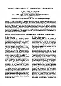
3 Shape spaces Shape spaces [4] were introduced in the context of the theoretical studies of clonal selection in the field of immunology. In this section we generalise the ideas underlying this methodology abstracting as many biological details as possible. A protein is composed of many different independent structural parts called domains. The interaction capability between domains depends on the structural and chemical complementarity of particular portions, called molecular determinants or motifs. Suppose it is possible to describe the features of a motif by specifying N “shape” parameters. These parameters include geometric quantities which specify the size and the shape of the molecular determinant, and physical characteristics of amino acids comprising the motif (e.g., the charge or the ability to form hydrogen bonds). The N parameters define an N -dimensional vector space that is called shape space, say S. A point in S represents a molecular determinant. A function C : S → S maps motif shapes to their complements. By defining a metric on S, the distance between two points can be used as a measure of interaction propension between two molecular determinants. N2 MA C(MB ) MB C N1 Figure 2: Shape space example

The above intuitions are sketched in Figure 2. We assume that two parameters N 1 and N2 suffice to describe molecular determinants, leading to a 2-dimensional shape space. Moreover we choose the Euclidean metric, obtaining an Euclidean shape space [10]. As an example, let us consider two proteins A and B, with molecular determinants M A and MB , respectively. The molecular determinants M A and MB are two points in the 2-dimensional Euclidean shape space. The function C : N1 × N2 → N1 × N2 maps MB into its complement C (MB ), and the distance ε =k MA − C (MB ) k represents the molecular affinity between the motifs M A and MB . In order to get symmetric interaction propension, one can require ε =k M A − C (MB ) k=k C (MA ) − MB k. If the N shape parameters do not contribute equally to the specificity of a motif (e.g. small charge differences could be more important than small differences in geometry), a metric different from the Euclidean one is required. Finding an appropriate metric for measuring the affinity of molecular determinants is a non trivial task in chemistry. The specific choice of the metric, however, does not affect our semantics. It is computationally difficult to calculate a distance in a high-dimensional continuous space. For this reason the abstract model of the shape spaces is not particularly well suited to a concrete implementation. Computational efficiency is gained by relying on strings and string matching rules to represent the affinity of motifs. Each motif is associated with a string of symbols, and hence a string can be loosely interpreted as 4

an amino acid sequence. Different symbols represent different values of properties of the amino acids, like, e.g., hydrophobicity or charge. To effectively compute the interaction propension between motifs it is necessary to define a string matching rule. Choosing the ‘right’ rule can be hard, and different biological situations might require different matching rules. Indeed quite a bit of distinct rules have been proposed in the literature, like, e.g., the Hamming distance and the Manhattan distance. The first is given by the number of positions in which two strings differ, while the Manhattan distance between two strings is the sum of the distances between their digits [11]. For example, let us fix the two strings “54” and “84”. Their Hamming distance is 1 (they only differ in the leftmost symbol), and their Manhattan distance is 3 (obtained as 8-5+4-4). Yet another definition of distance comes from the so-called xor rule. Each symbol in the string is represented as a binary number, and the distance between two strings is computed as the normalised sum of the digits of the xor of the two numbers. This last notion of distance is finer than the Hamming distance, and it is computationally more efficient than the Manhattan rule. The shape spaces that use strings and matching rules are globally called Hamming spaces.

A

B

C

Figure 3: Hamming space example

Figure 3 shows an example of the use of Hamming spaces. Three proteins A, B and C with one motif each are reported in the picture. Each motif is represented by an eight digit string, where each digit can be 1 (drawn as a rectangle) or 0 (drawn as a square). So the motifs of A, B, and C are 11010010, 10110001, and 10100101, respectively. Assume that the function C : {0, 1}8 → {0, 1}8 maps 0s to 1s and 1s to 0s. We adopt the Hamming distance and compare each pair of strings reading the digits from left to right. The mutual interaction propensions of A, B and C are then given by d A C (B ) = 4, dA C (C ) = 2 and dB C (C ) = 6, where dX C (Y ) stays for the distance between X and Y . Since the lowest distance value is d A C (C ) , we can conclude that the two proteins A and C have the greatest interaction propension in the considered set. For the sake of clarity, in the above example we made two choices that are not quite realistic from a biological point of view. First, we chose to evaluate strings from left to right, while proteins freely float in the living matter and therefore many other different kinds of interaction are possible. A more concrete model would define the value dX C (Y ) as the longest stretch of consecutive complementary bits [12]. Second, we assumed a direct map between the distance d X C (Y ) and the interaction propension between X and Y . More generally, one would need to define a map between distance and interaction propension [11].

4 Beta-binders graphically In this section we briefly recall Beta-binders and comment on the generalisation that allows a direct representation of shape spaces. We resort to a graphical presentation of the language and of its rules. The interested reader is referred to [3] for the mathematical details concerning notation and semantics. In the present paper we just point out the single modification that has to be applied to the original formalism to directly render the notion of distance. Beta-binders builds on the intuition that biological entities have an internal ‘process unit’ and an ‘interface’ exposed to the external environment. For example, a protein has a backbone and motifs for interacting 5

with the environment. A cell has a similar structure: it has a membrane whose proteins act as an interface, and a complex internal structure that responds to the external changes. This interpretation of cell is quite limited if we are studying a single cell, but in the context of the study of cellular populations, e.g. in immunology, this vision is acceptable [13]. Furthermore, the computations internal to cells have a high degree of parallelism and is not surprising that techniques from concurrency theory can be used for representing structural changes of the living matter. Specifically, the Beta-binders formalism encloses mobile processes [14] into active borders. These borders, that represent the interface of the described entity, are equipped with typed binders which are used for discriminating between allowed and disallowed interactions with the environment. The processes lying within the borders are made up of a limited number of operators, each corresponding to a distinct possible behaviour. Given a denumerable set of names (channels), the basic syntax of internal processes (ranged over by P , Q, . . .) and the semantic meaning associated with the various operators is given as follows: xhyi. P

can output the name y over x and subsequently act as P ;

x(y). P

can perform an input over x, bind the received datum to y, and then act as P ;

P |Q

behaves as P in parallel with Q; the two sub-processes can either run independently or synchronise; behaves as P | ! P , i.e., it can spawn infinitely many copies of P .

!P

Above, “synchronisation” corresponds to the matching of complementary actions, namely an input and an output over the same channel name. A few more operators are also used. They will be presented later on in this section. Beta-binders is equipped with an intuitive graphical representation. We now explain the computational rules of the formalism by showing their application to a running example. Firstly consider the following Beta-binders process, denoted as S 1 . x : {a1 , a2 } S1

=

u : {a1 }

v : {a2 }

x(y). P1 | xhzi. P2

uhwi. Q

v(w). R

(A1 )

(B1 )

(C1 )

System S1 is composed by three Beta-binders processes, called boxes: A 1 , B1 , and C1 . These boxes represent sub-components that run in parallel, and their distribution in the space is irrelevant (e.g., one could as well draw box C1 to the left of A1 ). Each box is equipped with a beta binder (i.e. an interface). For example, box A1 is given the binder x : {a1 , a2 }, named x and typed by the set of names {a 1 , a2 }. Inter-boxes communication In system S1 , box A1 can interact with either B1 or C1 . This is so because: • A1 can perform the input x(y) over the name x of its binder, B 1 can perform the output uhwi over the name u of its binder, and, since the types of x and u are not disjoint, these input and output can match; 6

• also, the types of x and of the binder v are not disjoint, and the output xhzi of A 1 can match the input v(w) of C1 . Let us consider the inter-communication between A 1 and B1 . It consumes the actions x(y) and uhwi, in the first and in the second box respectively, and leads to the following configuration. x : {a1 , a2 } S1 → S 2 =

u : {a1 }

v : {a2 }

P1 {w/y } | xhzi. P2

Q

v(w). R

(A2 )

(B2 )

(C1 )

Notice that the information w flowed from box B 1 of S1 to box A2 of S2 , represented by the substitution of the name w for the occurrences of y in P 1 , written P1 {w/y }. Intra-boxes communication In system S1 , a communication within box A1 is enabled as well. It would lead to the following configuration. x : {a1 , a2 } S1 → S 3 =

u : {a1 }

v : {a2 }

P1 {z/y } | P2

uhwi. Q

v(w). R

(A3 )

(B1 )

(C1 )

In the transformation S1 → S3 we observe an internal modification of the leftmost box from A 1 to A3 . The other two boxes remain unaffected. Given the initial system S 1 , inter-communication and intracommunication are both allowed to occur. This reflects real biological situations. For example, internal modifications of the structure of a protein are in competition with environmental solicitations, like, e.g., the interaction with an enzyme. Interface handling Internal processes are also provided with a limited number of operations for managing box interfaces. The associated syntax and semantics is described below: hide(x) . P

make the binder x invisible then behaves like P . (When made invisible, x is written x h .) If the enclosing box has no x-named binder, it stucks;

unhide(x) . P

make the binder xh visible then behaves like P . (When made visible again, xh is turned back to x.) If the enclosing box has no xh -named binder, it stucks;

expose(x, ∆) . P

add a x-named binder typed by ∆ then behaves as P . 7

Consider for instance the box D1 drawn below. xh : {a1 , a2 }

x : {a1 , a2 } hide(x) . expose(z, {b1 , b2 }) . P | Q

z : {b1 , b2 }

P |Q

→→

(D1 )

(D2 )

The execution of the prefix hide(x) hides the binder named x and changes its name to x h . Then the execution of the prefix expose(z, {b 1 , b2 }) adds to the box a new beta binder typed by {b 1 , b2 }. As a result of this, after two computational steps, D 1 is transformed into D2 . Notice that a box may be associated with more than one single binder, as it is the case for D 2 above. Indeed, unless otherwise specified, when talking about the “binder” of any given box, we refer to the set of all its singular binders. For instance, the binder of D 2 is the set composed of the two elements x h : {a1 , a2 } and z : {b1 , b2 }. Box joining and splitting To handle the box structure, Beta-binders is provided with operations for joining boxes together and for splitting one box in two. The join operation is parametric w.r.t. a function, called f join , and models different possible ways of merging boxes, each of them depending on a distinct instantiation of f join . Let B 1 , B 2 , B 0 stay for box binders, and let σ1 , σ2 represent name substitutions. Then, under the hypothesis that the actual function fjoin is defined at (B 1 , B 2 , P1 , P2 ) and that fjoin (B 1 , B 2 , P1 , P2 ) = (B 0 , σ1 , σ2 ), the general pattern of the join transformation can be graphically rendered as follows: B1

B0

B2 P1

P2

(E1 )

(E2 )

→

P1 σ1 | P 2 σ2 (E’)

The above transformation, just like those illustrated before, can be applied to a subset of a bigger system, leaving the rest unaffected. Namely, if the global system were made up of E 1 , of E2 , and of some other box E3 , then after the transformation the system would be composed of two boxes: E’ and E 3 . The operation that rules the splitting of boxes is dual to the above joining transformation. If fsplit (B, P1 , P2 ) = (B 1 , B 2 , σ1 , σ2 ) then a box with binder B and internal process P 1 | P2 is modified in two boxes: each of them with binder B i and internal process Pi σi , for i = 1, 2.

4.1 Integrating shape spaces into Beta-binders Beta-binders offers a natural ground for the integration of shape spaces. Essentially, in other process calculi interactions only depend on the matching of complementary actions (e.g., of an input and an output over the same channel). In Beta-binders the above requirement is partially relaxed and, at the level of interfaces, an input over x : ∆ can match whichever output over w : Γ, provided that ∆ and Γ share some common element. 8

Here the definition of types and their management is specialised further so to capture the intuition behind Hamming spaces and string matching rules. In particular, types become strings of names, and compatibility of types (originally interpreted as non-empty intersection of sets) becomes distance between strings. As it was observed in Section 3, distinct matching rules can best fit different contexts. Hence we adopt the following abstract definition of distance. Definition 4.1 Given two strings of symbols Γ and ∆ over the alphabet A, the distance function ρ(Γ, ∆) is a map An × Am → R, where n is the length of Γ, and m is the length of ∆. The definition of the distance function leaves the user free to use different matching rules, leaving the rest of the formal system unaffected. Consider for example the following boxes. x : a 1 a2 b1 b2 a1

u : a 1 a1 b1 b1 a1

x(k). P1 | P2

uhwi. Q1 | Q2

(F1 )

(F2 )

We can set to ∞ the distance between strings of different length, and assume symbols be complementary to themselves. Then, adopting the Hamming distance for strings of the same length, we get ρ(a1 a2 b1 b2 a1 , a1 a1 b1 b1 a1 ) = 2. In a quantitative context this value could be directly used for deriving specific stochastic parameters. In a qualitative view, one can say that the interaction between F 1 and F2 is allowed only if the distance between the types of their binders is lower than a given threshold (see [11] for some examples about this). Indeed, to directly deal with shape spaces, the formal rule defined in [3] for the inter-communication between a box with an elementary binder x : Γ and a box with an elementary binder y : ∆ is modified by requiring that: ρ(Γ, ∆) < threshold where “threshold” is a suitable user-defined value.

5 A simple model from the immune system We conclude the paper by showing how the above formalism can be applied to model the interactions of a few key players of the immune system. As an example, we consider a little system composed of a cell, a virus, and a cytotoxic T cell. First, we represent the three actors as boxes with appropriate binders. Then define suitable instances of the f join and of the fsplit functions that allow the modeling of cell infection, virus replication, and binding of T cells to infected cells. On passing, we show one of the possible runs of the whole system. The formal representation of the system is graphically given as follows: x : ∆C

y : ∆ V1

z : ∆ V2

w : ∆T

dna(x1 ). dna(x2 ). Cact

! dnaheV1 i. dnaheV2 i

T

(Cell)

(Virus)

(TCell)

9

(S1)

where ∆C = cabbaba, ∆V1 = vbaaaab, ∆V2 = vabbbabba, ∆T = tbaaabbbb, and Cact =! expose(y, x1 ). expose(z, x2 ). Also, for notational convenience, we use the following shorthands: C = dna(x 1 ). dna(x2 ). Cact , and V = ! dnaheV1 i. dnaheV2 i. Looking at the above specification of C act , notice that we use a name, rather than a set, as second parameter of the expose( , ) operator. This discrepancy w.r.t. the semantics presented in [3] can be motivated by supposing that some names are taken from a distinguished set in bijection with the set of the typing strings. Under the same assumption, the names e V1 and eV2 transmitted by Virus over dna are to be thought of as encodings of the types ∆ V1 and ∆V2 . Cell represents an eukaryote cell with a site x that expresses its interaction capabilities. The cell machinery is rendered by the input actions over dna that, when consumed, trigger C act and hence the exposition of new binders. Virus stays for an intracellular parasite. This kind of parasites consist of an outer cell (capsid) made up of proteins and of an interior core containing the genome (DNA or RNA). A virus can enter into a cell and, once inside, it uses the cell machinery to duplicate the genome and to synthesize proteins. In this way the virus builds a new capsid and a new core, i.e. it duplicates itself. The newly generated virus can exit the cell, while the originator still infects it. The Virus box is provided with two sites, the one typed by ∆ V1 is used to model cell infection, while the site typed by ∆ V2 can be recognised by highly specific lymphocytes (which are missing from the present picture). TCell represents a cytotoxic T cell of the adaptive immune responses. T cells circulate in the body searching for cells that have been infected by external organisms, like viruses. In fact, infected cells display on their surfaces some fragments of the viral proteins. A T cell that recognises an infected cell kills it, so preventing the diffusion of the virus. T cells are highly specific and hence they require a high affinity with the virus fragment displayed by the infected cell. The binder types we use in our model are strings that encode the representation of the box they belong to. In the above model, the alphabet of the typing strings is {c, v, t, a, b}. The first symbol of the string encodes the owner of the binder associated with that type: c stays for Cell, v for Virus, and t for TCell. The rest of any typing string, that actually represents the shape of the binder, is made up of as and bs. We assume that the complementarity function C : Am → Am behaves as the identity on the elements of the set {c, v, t} and maps as to bs and bs to as. Letting H( , ) denote the Hamming distance, we now define the distance function as follows: ρ(x∆, yΓ) =

if m =| ∆ |=| Γ | and ∆ ∈ {a, b} m and Γ ∈ {a, b}m then H(∆, C (Γ)) else max (| ∆ |, | Γ |).

Notice that the first symbol of each of the two strings, representing the class of the binder rather than its shape, is ignored. Also observe that ρ(∆ C , ∆V1 ) = H(abbaba, C (baaaab)) = 1, meaning that the affinity between the binder of Cell and the virus binder named y is high. We now complete the specification of our model by defining the functions that rule the joining and splitting of boxes. In what follows, the metavariables B ∗ , B ∗1 , B ∗2 , . . . are used to denote possibly empty box binders. The first rule, driven by an instance of f join called fjoin VC , can be graphically rendered as follows.

10

B ∗1 if ρ(vΓ, c∆) < 3

(fjoin VC )

B ∗2

y : vΓ P1

B ∗2

x : c∆ P2

→

x : c∆

P1 | P 2

The rule states that, if in the global system there are two boxes which exhibit binders typed by vΓ and by c∆, respectively, and if the distance between these two types is less than 3, then the two boxes can be joined together and the resulting box has the same binder as the c∆-typed box. When applicable, this rule models cell infection. In particular, starting from the global system S1, we get: x : ∆C S1 →

w : ∆T

C|V

x : ∆C

T

y : ∆ V1

z : ∆ V2

Cact σ | V

→→→→

w : ∆T T

(S2)

where σ = {eV1/x1 , eV2/x2 }. In the above, the first computational step is due to the f join VC transformation that makes the virus genetic material V enter the cell. The following computational steps correspond to intra-communications over dna and to the subsequent exposition of the received binder types. Referring to S2, observe that Cact σ = ! expose(y, eV1 ) . expose(z, eV2 ) can keep exposing the virus proteins an unlimited number of times. So the cell never gets “consumed” by the virus. As outlined in [3], a slight refinement of the formal model could take care of this aspect and limit the number of possible replications of the process expose(y, e V1 ) . expose(z, eV2 ). We now define the rules for virus replication and for the binding of T cells to infected cells, which are driven by fsplit VC and fjoin CT , respectively. y : vΓ

B (fsplit VC )

z : v∆

Cact σ | V

→

B ∗1 (fjoin CT )

if ρ(tΓ, v∆) < 2

w : tΓ P1

y : vΓ

B

B ∗2

z : v∆

Cact σ

V

y : v∆

B ∗1 B ∗2 wh : tΓ

Cact σ

→

P1 | Cact σ

We conclude this section by showing one of the possible computations that can be automatically derived from S2. The computation reflects the application of the following sequence of transformations: f split VC , exposition of the ∆V1 and ∆V2 -typed binders by the infected cell, and f join CT transformation. 11

x : ∆C Cact σ

S2 →

x : ∆C

y : ∆ V1

T

z : ∆ V2

w : ∆T

Cact σ

→→ x : ∆C →→

w : ∆T

y : ∆ V1

T w h : ∆T

z : ∆ V2

Cact σ | T

y : vΓ

z : v∆

V

y : vΓ

z : v∆

V y : vΓ

z : v∆

V

5.1 Compositionality to hammer complexity One of the main advantages in using formal methods and process calculi theory comes from compositionality. Compositionality means that it is possible to develop different pieces of a model separately and then putting all together following mathematical rules. The underlying idea is to see biomolecular (as well as cellular) systems as a set of elementary components from which complex entities are constructed. This introduces a new paradigm with respect to “classical” complex biological system modeling. Indeed immunologists are moving in this direction, leaving differential equations models for agent based model [15] or stochastic stage-structured model [13]. But the new models lack in strong mathematical backgrounds, that seems a mandatory requirement for modeling, analysing and sharing biological knowledge. In this section we realise this idea developing a simple model of an antibody and showing how it can be integrated in the model we presented above. An antibody is a molecule that has a specialised portion for identifying other molecules called paratope. Paratope has a defined shape that characterises the molecules that it can interact with. Each foreign molecule (e.g. viruses) presents a certain relief or pattern that can be recognised with various degrees of precision by complementary patterns or paratopes located on antibody molecules. When an antibody A recognises a virus V , it happens that A binds V preventing infection. Moreover the newly generated complex A − V has a new binder that helps phagocytic cell. For instance, the capsule that surrounds pneumococci protects them from phagocytosis. If the appropriate antibodies are present in the body, they combine with the capsule and now the pneumococci can be ingested [16]. The formal representation of an antibody is graphically described below: k : ∆A A (AntyB)

12

where ∆A = pabbbba. Also we have to define the function that drives the joining of a virus and an antibody. B ∗1

z : vΓ1 y : vΓ2 if ρ(vΓ, a∆) < 2

(fjoin VA )

P1

z : vΓ1 B ∗1 x : m∆M

x : p∆ P2

P1 | P 2

→

The above rule states that, if there is an antibody that is able to recognise a virus, then the antibody binds it. The new complex is no more able to enter in a cell and moreover a new binder x : m∆ M is added. This binder has high affinity with phagocytic cells helping the complex ingestion. Once defined the antibody model we can extend the system (S1) leading to: x : ∆C

y : ∆ V1

z : ∆ V2

w : ∆T

k : ∆A (S10 )

C

V

T

A

(Cell)

(Virus)

(TCell)

(AntyB)

This system can perform the same sequence of transformations depicted in the previous section, without any differences. Moreover the antibody can bind to the virus so preventing cell infection. x : ∆C S10 →

y : ∆ V2 z : ∆ M V |A

C (Cell)

(Virus+AntyB)

w : ∆T T (TCell)

Notice that the complex (Virus-AntyB) is no longer able to interact with (Cell). Moreover it is possible to automatically infer all the possible future behaviours of the system, giving a powerful methodology for investigating complex systems.

6 Conclusions and perspectives We presented a formalism to model complex (biological) systems. The main objective is to determine the suitable abstraction to have a formal description of systems on top of which analysis and simulation can be implemented. We selected here the biological applicative domain and in particular the immune systems because handling these phenomena could help us to control, design and program complex systems as well as to re-construct systems from incomplete data. The main achievement of the present work with respect to the definition of Beta-binders is the inclusion in the formalism of the representation of shape spaces. This enhancement shows how the formalism proposed is flexible in specifying systems at different levels of abstraction. We worked out also the main feature of compositionality showing how a system 13

can be specified incrementally by simply adding new descriptions to the ones already produced when new information becomes available. We are confident that this is a first step towards a theory of complex systems whose main brick is formal semantics of programming languages for concurrency (specifically process calculi). The study of process calculi and their definition since the beginning inspired by biological phenomena could lead to new biomimetic computational paradigms and primitives. The main goals of the new specification languages are to implicitly handle complexity in their semantic definition and to model, analyse, simulate and compare different systems. We feel this step very important because the major big step in research has been performed in the past when difficult concepts have been abstracted into good linguistic frameworks. Furthermore, the hierarchical nature of biological systems allows us to exploit the relation macro-world, meso-world and micro-world as a compilation problem. The impact of the above mentioned strategy is for sure on the life science side by helping biologists in their research, but also on the computer science side defining new techniques able to handle systems more complex than the actual ones. Furthermore the abstraction of biological models in terms of interaction/communication of active entities can help enhancing the understanding of many fields of computer science, besides of course complex systems theory. We mention here just two of them because are of relevant interest nowadays. Global computing and global computer have similar properties to biological systems because they are made up of autonomous and widely dispersed entities not centrally controlled, they include mobile code and appliances whose configurations vary over time and have incomplete information on the environment in which they work. If we can devise formalisms to handle biological systems, then we have good chances to improve the global computing field as well. The particular application of immune system design, analysis and simulation could lead to new ideas for developing information security framework that are self-adapting to the new context in which a treat is ongoing. Summing-up, we hope that the development of the present paper could lead to a larger applicability of the formalism presented in many different fields. In fact the abstraction molecules as processes and interaction as communication can be applied to any system whose evolution step is an interaction of some kind.

References 1. Gillespie D: A general method for numerically simulating the stochastic time evolution of coupled chemical reactions. J Comput Phys 1976, 22. 2. Priami C, Regev A, Silverman W, Shapiro E: Application of a stochastic passing-name calculus to representation and simulation of molecular processes. IPL 2001, 80. 3. Priami C, Quaglia P: Beta binders for biological interactions. In CMSB ’04, Volume 3082 of LNBI. Edited by Danos V, Sch¨achter VV, Springer 2005. 4. Perelson AS, Oster GF: Theoretical studies of clonal selection: minimal antibody repertoire size and reliability of self-non-self discrimination. J Theor Biol 1979, 81(4). 5. Regev A, Shapiro E: Cells as Computations. Nature 2002, 419. 6. Danos K, Krivine J: Formal molecular biology done in CCS-R. In BioConcur ’03 2005. 7. Regev A, Panina E, Silverman W, Cardelli L, Shapiro E: BioAmbients: An Abstraction for Biological Compartments. TCS 2004, 325.

14

8. Cardelli L: Brane Calculi. In CMSB ’04, Volume 3082 of LNBI. Edited by Danos V, Sch¨achter VV, Springer 2005. 9. Alberts B, Johnson A, Lewis J, Raff M, Roberts K, Walter P: Molecular biology of the cell (IV ed.). Garland science 2002. 10. Smith D, Forrest S, Hightower R, Perelson A: Deriving shape-space parameters from immunological data. J Theor Biol 1997, 189. 11. Detours V, Sulzer B, Perelson AS: Size and Connectivity of the Idiotypic Network Are Independent of the Discreteness of the Affinity Distribution. J Theor Biol 1996, 183. 12. De Boer RJ, Perelson AS: Size and connectivity as emergent properties of a developing immune network. J Theor Biol 1991, 149. 13. Chao D, Davenport M, Forrest S, AS P: A stochastic model of cytotoxic T cell responses. J Theor Biol 2004, 228. 14. Milner R: Communicating and Mobile Systems: the π-calculus. Cambridge Univ. Press 1999. 15. Seiden P, Celada F: A Model for Simulating Cognate Recognition and Response in the Immune System. J Theor Biol 1992, 158. 16. Wood W, Smith M, Watson B: Studies on the Mechanism of Recovery in Pneumococcal Pneumonia. J Exp Med 1946, 84:387.

15