SHARED FEATURE REPRESENTATIONS OF LIDAR AND OPTICAL IMAGES: TRADING SPARSITY FOR SEMANTIC DISCRIMINATION Manuel Campos-Taberner1 , Adriana Romero2 , Carlo Gatta3 and Gustau Camps-Valls1 ∗ † 1
Universitat de Val`encia, Spain. {manuel.campos,gustau.camps}@uv.es 2 Universitat de Barcelona, Spain.
[email protected] 3 Universitat Aut`onoma de Barcelona, Spain.
[email protected] ABSTRACT
This paper studies the level of complementary information conveyed by extremely high resolution LiDAR and optical images. We pursue this goal following an indirect approach via unsupervised spatial-spectral feature extraction. We used a recently presented unsupervised convolutional neural network trained to enforce both population and lifetime sparsity in the feature representation. We derived independent and joint feature representations, and analyzed the sparsity scores and the discriminative power. Interestingly, the obtained results revealed that the RGB+LiDAR representation is no longer sparse, and the derived basis functions merge color and elevation yielding a set of more expressive colored edge filters. The joint feature representation is also more discriminative when used for clustering and topological data visualization. 1. INTRODUCTION Image fusion of optical and LiDAR images is currently a successful and active field [1–5]. Intuition and physics tell us that both modalities represent objects in the scenes in different semantic ways: color versus altitude, or passive radiance versus active return intensity. But, is there a fundamental justification for this in statistical terms? Answering such question directly would imply measuring mutual information between data modalities. However, the involved random variables (i.e. RGB and LiDAR imagery) are multi-dimensional, they do have spatial structure, and do reveal distinctive spatial-spectral feature relations. Measuring multidimensional dependencies is not at all easy. We follow an indirect pathway: to analyze spatial-spectral feature representations with convolutional neural networks using RGB, LiDAR and the RGB+LiDAR shared representation. Such feature representations will be analyzed in terms of sparsity, compactness, topological visualization and discrimination ca∗ This work was partially funded by the Spanish Ministry of Economy and Competitiveness, under the LIFE-VISION project TIN2012-38102-C03-01. The work of A. Romero is supported by an APIF-UB grant. The work of C. Gatta is supported by MICINN under a Ramo´on y Cajal Fellowship. † The authors would like to thank the Belgian Royal Military Academy for acquiring and providing the data used in this study, and the IEEE GRSS Image Analysis and Data Fusion Technical Committee.
pabilities. The answer to the question is in the title of the contribution: combination of RGB+LiDAR leads to denser and less compact representations yet more discriminative: such feature “orthogonality” in nonlinear statistical terms explains the success of the joint use. The statistical properties of very high resolution (VHR) and multispectral images place important difficulties for automatic analysis, because of the high spatial and spectral redundancy, and their potentially non-linear nature1 . Beyond these well-known data characteristics, we should highlight that spatial and spectral redundancy also suggest that the acquired signal may be better described in sparse representation spaces, as recently reported in [7,8]. Seeking for sparsity may in turn be beneficial to deal with the increasing amount of data due to improvements in spatial resolution. Learning expressive spatial-spectral features from images in an efficient way is thus of paramount relevance. Moreover, learning such features in an unsupervised fashion is an even more important issue. In recent years, dictionary learning has emerged as an efficient way to learn sparse image features in unsupervised settings, which are eventually used for image classification and object recognition: discriminative dictionaries have been proposed for spatial-spectral sparse-representation for image classification [9,10], sparse bag-of-words codes for automatic target detection [11], and unsupervised learning of sparse features for aerial image classification [12]. Most of the methods describe the input images in sparse representation spaces but do not take advantage of the high non-linear nature of convolutional neural networks (CNN) architectures. In this paper we introduce the use of unsupervised feature learning with CNNs with the goal of studying the statistical properties of joint RGB+LiDAR representation spaces. The remainder of the paper is organized as follows. Section 2 reviews the proposed algorithm for unsupervised feature learning using CNN that enforces sparse representations. Section 3 describes the data used, and Section 4 presents and discuss our main findings. Section 5 concludes with a few remarks. 1 Factors such as multi-scattering in the acquisition process, heterogeneities at subpixel level, as well as atmospheric and geometric distortions lead to distinct non-linear feature relations, since pixels lie in high dimensional curved manifolds [6, 7].
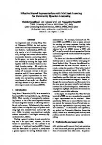
2. UNSUPERVISED FEATURE LEARNING WITH CONVOLUTIONAL NETWORKS Convolutional Neural Networks (CNN) consist of several layers stacked on top of each other, such that the output of a layer is used as input of the next layer. The input of the first layer is the given data, in this case a hyper-spectral image. One layer is composed of three parts: (1) a set of convolutional linear filters, whose parameters can be learned by means of unsupervised or supervised techniques; (2) a point-wise nonlinearity, e.g. the logistic function; and (3) a pooling operation, e.g. a non-overlapping 2 × 2 sliding window computing the maximum of its input (called max-pooling). The rationale of these three parts is (1) to provide a simple local feature extraction; (2) to modify the result in a non-linear way to allow the CNN architecture to learn non-linear representations of the data; and (3) to reduce the computational cost and provide a certain local translational invariance. As stated before, we train the CNN to extract sparse representations. Intimately related to our method, Orthogonal Matching Pursuit (OMP-k) [13] extracts sparse feature representations by training a network in an unsupervised fashion. OMP-k trains a set of filters by iteratively selecting an output of the code to be made non-zero in order to minimize the residual reconstruction error, until at most k outputs have been selected. The method achieves a sparse representation of the input data in terms of population sparsity. SAE trains the filters by minimizing the reconstruction error while ensuring similar activation statistics through all training samples among all outputs, thus ensuring a sparse representation of the data in terms of lifetime sparsity. In this paper, we use the EPLS algorithm [14], which iteratively builds a sparse output target and optimizes for that specific target to learn the filters of each layer. The sparse target is defined such that it represents each sample with one “hot code” and ensures the same mean activation among all outputs. Using this approach, we obtain a sparse feature representation of the data, in terms of both population and lifetime sparsity. The CNN trained with the EPLS is computationally very efficient and leads to sparse representations. Here we use this method to analyze the hidden and shared representations learned from the data by a CNN, see Fig. 1. Note that the shared RGB+LiDAR representation is made of non-linear spatial and spectral combinations of input RGB and LiDAR features.
Fig. 1. Considered independent (a) RGB and (b) LiDAR representations, along with the (c) shared RGB+LiDAR representation.
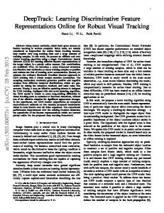
3. DATA COLLECTION The 2015 IEEE GRSS Data Fusion Contest delivers extremely high resolution LiDAR and color orthophotos2 . The imaging data were acquired on March 13, 2011, using an airborne platform flying at the altitude of 300 m over the urban and the harbor areas of Zeebruges, Belgium (51.33 N, 3.20 E). The data were collected simultaneously and were georeferenced to WGS-84. The point density for the LiDAR sensor was approximately 65 points/m2 , which is related to point spacing of approximately 10 cm. We will use the derived digital surface model (DSM) in the study. The color orthophotos were taken at nadir and have a spatial resolution of approximately 5 cm. The data set is organized into 7 separate tiles. The color orthophotos are 10000×10000 pixel-sized, while the DSM is 5000×5000 pixel-sized. Fig. 2 shows both images for the first tile, in which we will focus here.
Fig. 2. RGB (5 cm/pix) and LiDAR (10 cm/pix) images provided in the IEEE GRSS competition 2015.
4. EXPERIMENTAL RESULTS In this section, we study the information content captured by a convolutional neural network (CNN) trained to enforce sparsity with EPLS in the three scenarios: RGB, LiDAR and joint RGB+LiDAR. Several analyses are done: we pay attention to the lifetime and population sparsity scores as a measure of compactness of the represenations. Then, we visualize the learned representations in a topological space. Finally, we study the discriminative power of the extracted features when used for image segmentation. 4.1. Experimental setup We show results for the first tile, for which we generated 100,000 image patches of size 10×10. A total number of 30,000 images patches were used for training all networks. In all three situations, we trained the CNNs using a maximum of NH = 1000 hidden nodes. For all the architectures, we tried several symmetric receptive fields (of sizes 3 × 3 and 5 × 5, 7 × 7, 10 × 10 pixels). We trained the networks on contrastnormalized image patches by means of EPLS with logistic non-linearity and retrieve the sparse features by applying the 2 http://www.grss-ieee.org/community/technical-committees/datafusion/data-fusion-contest/
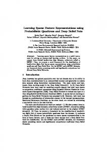
network parameters with natural encoding (i.e. with the logistic non-linearity) and polarity split. 4.2. On the sparsity of the learned representations After training CNN in the three situations, we studied both the Lifetime sparsity (LS), and the Population sparsity (PS). Figure 3 shows the obtained results. One can see that by adding LiDAR to RGB, lifetime sparsity is increased, independently of the receptive field (RF) used. Note that the lower the value of LS, the closer to the objective of maintaining similar mean activation among outputs. The learned representation is thus no longer sparse, which suggests that RGB and LiDAR carry orthogonal information and thus it is more difficult to obtain a compact representation. Similar trends are obtained for NH , but only for high values, say NH > 100, which can be due to the poor representation in general obtained for low values of NH (big errors, results not shown). On the contrary, by adding LiDAR to RGB, PS is reduced for any RF and NH value. The same reasoning as before holds here. Population sparsity captures that a small subset of outputs are very active at the same time. This does not happen when merging RGB+LiDAR because these features convey complementary information and hence a great many features activate simultaneously. 450
0.4 RGB LiDAR RGB+LiDAR
0.35
350 Population sparsity
Lifetime sparsity
0.3 0.25 0.2 0.15 0.1
300 250 200 150 100
0.05 0 3
RGB LiDAR RGB+LiDAR
400
50 4
5
6
7
8
9
0 3
10
1.4
5
6
7
8
9
10
450
RGB LiDAR RGB+LiDAR
1.2
4
RF
RF
RGB LiDAR RGB+LiDAR
400 350 Population sparsity
Lifetime sparsity
1 0.8 0.6
300 250 200 150
0.4 100
0.2 0 1 10
50 2
10 NH
3
10
0 1 10
2
10 N
3
10
H
Fig. 3. Lifetime and population sparsity for RGB, LiDAR and RGB+LiDAR as a function of the receptive field (top) and the number of hidden neurons (bottom).
4.3. On the topology of the learned representations Figure 4 shows the learned bases by the convolutional net using EPLS for RGB, LiDAR and RGB+LiDAR (top), and the corresponding topological representations via projection on the first two ISOMAP components (bottom). We intentionally fixed the neighborhood size to k = 1 in ISOMAP’s epsilon distance. The EPLS algorithm applied to very high resolution color images learns not only common bases such
Fig. 4. Learned bases by the convolutional net using EPLS for RGB, LiDAR and RGB+LiDAR (top), and the corresponding topological representations via projection on the first two ISOMAP components (bottom). as oriented edges/ridges in many directions and colors, but also corner detectors, tri-banded colored filters, center surrounds and Laplacian of Gaussians among others [14]. This suggests that enforcing lifetime sparsity helps the system to learn a set of complex and rich bases. On the other hand, the learned LiDAR bases are edge detectors related to ‘changes in height’ of the objects, e.g. containers-vs-ground, roof-vsground, ground-vs-sea, roofs, train rails vs. ground in the image. When combining RGB+LiDAR, the learned bases inherite properties of both modalities, resembling altitudecolored detectors. For the projections onto the first two ISOMAP components, we can see that RGB bases scatter twofold: a colorpredominant diagonal on top of a typical edges and tri-band grayscale textures. Higher frequency (both grayscale and colored) lie far from the subpsace center. For LiDAR the scatter is much simpler: low frequencies in the center and heightedges surrounding the center of the subspace. When RGB and LiDAR are combined, color and texture clusters are disentangled, but height-edges become a bit more colored, and again high-frequency patterns lie far from the mean. 4.4. On the discriminative power of the representations An alternative way to analyze the extracted features and their complementarity is to use them for clustering. We run the standard k-means on top of the extracted features for different degrees of granularity, k = 2, . . . , 20. Fig. 5[left] shows the classification maps for k = 10. It should be noted that RGB dominates many clusters in the joint/shared representation. Nevertheless, the RGB+LiDAR map shows new emerging groups of semantic clusters, e.g. harbor cranes close the sea. Some other clusters are just inherited from the individual LiDAR solution, e.g. big buildings with constant height. The quality of clustering solutions is a controversial issue and many techniques exist in the literature to evaluate
RGB
LiDAR
RGB+LiDAR Davies−Bouldin index 1
Dunn index
2
RGB LiDAR RGB+LiDAR
0.8
10
RGB LiDAR RGB+LiDAR
1
10
0.6 0
10
0.4 −1
10
0.2
0 0
−2
5
10 k clusters
15
20
10
0
5
10 k clusters
15
20
Fig. 5. Clustering using k-means on top of the CNN features (left) and validity indices as a function of k (right). clustering solutions. The general idea in all of them is to favour compact and distant clusters. Figure 5[right] shows the Davies-Bouldin and the Dunn’s validity indices as a function of k (similar results where obtained for the R2 and the Calinski-Harabasz indices, not shown). Results suggest that the joint representation leads to similar solutions to those obtained with RGB alone, yet resemble more semantically expressive.
[3]
[4]
5. CONCLUSIONS [5]
This paper presented a study on the level of complementary information conveyed by extremely high resolution LiDAR and optical images. We analyzed the expressive power and richfulness of extracted features from RGB, LiDAR and RGB+LiDAR using state-of-the-art unsupervised learning. In particular, we used a recently presented unsupervised convolutional neural network that aims to learn feature representations that are sparse. This distinct characteristic of the algorithm has revealed very useful in semantic segmentation of images. However, in our experiments, the combination of RGB and LiDAR has given rise to a feature representation that is no longer sparse according to different sparsity scores, thus suggesting that RGB and LiDAR convey ‘orthogonal’ and complementary pieces of information. Beyond the focus on sparsity, we also payed attention to the induced topological spaces through ISOMAP embeddings. The analysis again revealed interesting complementarity: RGB combined with LiDAR leads to more semantic representations in which color and altitude are combined to better object description. The obtained joint feature representation suggests a kind of semantic extraction. The orthogonality in information does not only come out in terms of lack of sparse solutions, but also in terms of discimination, as it was studied through image segmentation, where more expressive and semantic maps emerge.
[6]
[7]
[8]
[9]
[10]
[11]
[12] 6. REFERENCES [1] B. Koetz, G. Sun, F. Morsdorf, K. Ranson, M. Kneubhler, K. Itten, and B. Allgwer, “Fusion of imaging spectrometer and LiDAR data over combined radiative transfer models for forest canopy characterization,” Rem. Sens. Envir., vol. 106, no. 4, pp. 449 – 459, 2007. [2] A. F. Elaksher, “Fusion of hyperspectral images and LiDAR-
[13]
[14]
based dems for coastal mapping,” Optics and Lasers in Engineering, vol. 46, no. 7, pp. 493 – 498, 2008. A. Swatantran, R. Dubayah, D. Roberts, M. Hofton, and J. B. Blair, “Mapping biomass and stress in the sierra nevada using lidar and hyperspectral data fusion,” Rem. Sens. Envir., vol. 115, no. 11, pp. 2917 – 2930, 2011. L. Naidoo, M. Cho, R. Mathieu, and G. Asner, “Classification of savanna tree species, in the Greater Kruger National Park region, by integrating hyperspectral and LiDAR data in a random forest data mining environment,” ISPRS Jour. Photogram. Rem. Sens., vol. 69, no. 0, pp. 167 – 179, 2012. M. Pedergnana, P. Marpu, M. Dalla Mura, J. Benediktsson, and L. Bruzzone, “Classification of remote sensing optical and LiDAR data using extended attribute profiles,” IEEE Jour. Sel. Top. Sig. Proc., vol. 6, no. 7, pp. 856–865, Nov 2012. G. Camps-Valls, D. Tuia, L. G´omez-Chova, S. Jim´enez, and J. Malo, Eds., Remote Sensing Image Processing. LaPorte, CO, USA: Morgan & Claypool Publishers, Sept 2011. G. Camps-Valls, D. Tuia, L. Bruzzone, and J. Atli Benediktsson, “Advances in hyperspectral image classification: Earth monitoring with statistical learning methods,” Signal Processing Magazine, IEEE, vol. 31, no. 1, pp. 45–54, Jan 2014. R. Willett, M. Duarte, M. Davenport, and R. Baraniuk, “Sparsity and structure in hyperspectral imaging: Sensing, reconstruction, and target detection,” IEEE Sig. Proc. Mag., vol. 31, no. 1, pp. 116–126, Jan 2014. Z. Wang, N. Nasrabadi, and T. Huang, “Spatial-spectral classification of hyperspectral images using discriminative dictionary designed by learning vector quantization,” IEEE Trans. Geosc. Rem. Sens., vol. 52, no. 8, pp. 4808–4822, Aug 2014. S. Yang, H. Jin, M. Wang, Y. Ren, and L. Jiao, “Data-driven compressive sampling and learning sparse coding for hyperspectral image classification,” IEEE Geosc. Rem. Sens. Lett., vol. 11, no. 2, pp. 479–483, Feb 2014. H. Sun, X. Sun, H. Wang, Y. Li, and X. Li, “Automatic target detection in high-resolution remote sensing images using spatial sparse coding bag-of-words model,” IEEE Geosc. Rem. Sens. Lett., vol. 9, no. 1, pp. 109–113, Jan 2012. A. Cheriyadat, “Unsupervised feature learning for aerial scene classification,” IEEE Trans. Geosc. Rem. Sens., vol. 52, no. 1, pp. 439–451, Jan 2014. A. Coates and A. Ng, “The importance of encoding versus training with sparse coding and vector quantization,” in ICML, 2011, pp. 921–928. A. Romero, P. Radeva, and C. Gatta, “Meta-parameter free unsupervised sparse feature learning,” IEEE Trans. Patt. Anal. Mach. Intell., 2014, accepted.