Jun 20, 2016 - ... success these. arXiv:1602.01448v2 [physics.data-an] 20 Jun 2016 ... or vibrations. Here, we describe an algorithm approach and software.
LBNL-1003977
SHARP: a distributed, GPU-based ptychographic solver Stefano Marchesini,1 Hari Krishnan,1 David A. Shapiro,1 Talita Perciano,1 James A. Sethian,1 Benedikt J. Daurer,2 and Filipe R.N.C. Maia2
arXiv:1602.01448v1 [physics.data-an] 30 Jan 2016
1
Lawrence Berkeley National Laboratory, Berkeley, CA, USA 2 Uppsala University, Uppsala, Sweden (Dated: February 4, 2016)
Ever brighter light sources, fast parallel detectors, and advances in phase retrieval methods, have made ptychography a practical and popular imaging technique. Compared to previous techniques, ptychography provides superior resolution at the expense of more advanced and time consuming data analysis. By taking advantage of massively parallel architectures, high-throughput processing can expedite this analysis and provide microscopists with immediate feedback. These advances allow real-time chemical specific imaging at wavelength limited resolution, coupled with a large field of view. Here, we introduce a set of algorithmic and computational methodologies, packaged as an open source software suite, aimed at providing state-of-the-art high-throughput ptychography reconstructions for the coming era of diffraction limited light sources.
I.
INTRODUCTION
Reconstructing the 3D map of the scattering potential of a sample from measurements of its far-field scattering patterns is an important problem. It arises in a variety of fields, including optics [1, 2], astronomy [3], Xray crystallography [4], tomography [5], holography [6, 7] and electron microscopy [8]. As such it has been a subject of study for applied mathematicians for over a century. The fundamental problem consists of finding the correct phases that go along with the measured intensities, such that together they can be Fourier transformed into the real-space image of the sample. To help recover the correct phases from intensity measurements a range of experimental techniques have been proposed along the years, such as interferometry/holography [6, 7], gratings [9], random phase masks and many others [10–20]. Progress has been made in solving the phase problem for a single diffraction pattern recorded from a nonperiodic object[21–25]. Such methods, referred to as coherent diffractive imaging (CDI), attempt to recover the complete complex-valued wave scattered from the object, providing phase contrast as well as a way to overcome depth-of-focus limitations of regular optical systems. Ptychography, a relatively recent technique, provides the unprecedented capability of imaging macroscopic specimens in 3D and attain wavelength limited resolution (i.e. potentially atomic resolution) along with chemical specificity. Ptychography was proposed in 1969 [26–30] with the aim of improving the resolution in x-ray and electron microscopy. Since then it has been used in a large array of applications, and shown to be a remarkably robust technique for the characterization of nano materials [26, 27, 29, 31–51]. Ptychography can be used to obtain large highresolution images. It combines the large field of view of a scanning transmission microscope with the resolution of scattering measurements. In a scanning transmission microscope a focused beam is rastered across a sample, and the total transmitted intensity is recorded for each
beam position. The pixel positions of the image obtained correspond to the beam positions used during the scan, and the value of the pixel to the intensity transmitted at that position. This limits the resolution of the image to the size of the impinging beam, which is typically limited by the quality of focusing optics and work distance constraints. In ptychogrpahy, instead of only using the total transmitted intensity, one typically records the distribution of that intensity in the far-field, i.e. the scattering pattern produced by the interaction of the illumination with the sample. The diffracted signal contains information about features much smaller than the size of the x-ray beam, making it possible to achieve higher resolutions that with the scanning techniques. The downside of using the intensities is that one now has to retrieve the corresponding phases to be able to reconstruct an image of the sample, which is made even more challenging by the presence of noise, experimental uncertainties, and perturbations of the experimental geometry. Ptychographical phasing is a non-linear optimization problem still containing many open questions [52]. While it is a difficult problem, it is usually tractable by making use of the redundancy inherent in obtaining diffraction patterns from overlapping regions of the sample. This redundancy also permits the technique to overcome the lack of several experimental parameters and measurement uncertainties. For example, there are methods to recover unknown illuminations [29, 33, 34, 36, 53]. As a testament to their success these methods are even used as a way of characterizing high quality x-ray optics [37–39], the wavefront of x-ray lasers [54] and space telescopes [55]. Several strategies, such as Alternating Directions [56], projections, gradient, conjugate gradient, Newton [57], spectral methods [46, 52, 58], and Monte-carlo [40], have been proposed to handle situations when both sample and illumination function, positions, are unknown parameters in high dimensions, and to handle experimental situations such as partial coherence, background, averaging during flying scans, vibrations[3, 40–44, 57–63]
2 a(1) (q)
py
y
a(K) (q)
ordinates
p
q = kout − kin � � 1 √(px2 ,py 2,zD )2 − (0, 0, 1) = px +py +zD λ 1 ' (px , py , 0) λzD
px
x
FIG. 1. Experimental geometry in ptychography: an unknown sample with transmission ψ(r) is rastered through an illuminating beam ω(r), and a sequence of diffraction measurements I(i) = |a(i) (q)|2 are recorded on an area detector with pixel coordinates p at a distance zD from the sample.
Here we describe an algorithm approach and open software suite “sharp” (Scalable Hetereogeneous Adaptive Real-time Ptychography) that enables high throughput streaming analysis using computationally efficient phase retrieval algorithms. The high performance computational back-end is hidden from the microscopist, but can be accessed and adapted to particular needs by using a python interface or by modifying the source code. Using “sharp” we have built an intuitive graphical user interface that provides visual feedback, of both the recorded diffraction data as well as the reconstructed images, throughout the data aquisition and reconstruction processes at the ALS.
II.
p are the incident where kin = (0, 0, k) and kout = k |p| and scattered wave vectors that satisfy |kin | = |kout | = k = 1/λ, and λ is the wavelength. With a distance pm from the center to the edge of the detector, the diffraction limited resolution (half-period) of the microscope is D given by the lengthscale r = λz 2pm . As a consequence, the coordinates in reciprocal and real space are defined as � µ ν q = mr , mr , µ, ν ∈ {0, . . . , m − 1}
and r = (rµ, rν) , µ, ν ∈ {0, . . . , m − 1}, x(i) = (rµ0 , rν 0 ) , µ0 , ν 0 ∈ {0, . . . , n − m}. While x(i) is typically rastered on a coarser grid, r + x(i) spans a finer grid of dimension n × n. In other words, we assume that a sequence of k diffraction intensity patterns I(i) (q) are collected as the position of the object is rastered on the position x(i) . The p simple transform a(i) = I(i) (q) is a variance stabilizing transform for Poisson noise [64, 65]. The relationship among the amplitude a(i) (q), the illumination function w(r) and an unknown object ψ(r) to be estimated can be expressed as follows:
SHARP SOFTWARE SUITE
a(i) (q) = Fw(r)ψ(r + x(i) ) Forward model
In a ptychography experiment (see Fig. 1), one performs a series of diffraction measurement as a sample is rastered across an x-ray beam. The illumination is formed by an x-ray optic such as a zone-plate. The measurement is performed by briefly exposing an area detector such as a CCD which records the scattered photons. In a discrete setting, a two-dimensional small beam with distribution w(r) of dimension mx × my illuminates a subregion centered at x(i) (referred to as frame) of an unknown object of interest ψ(r) of dimension nx × ny . Here 0 < m < n, i = 1, . . . , K and K is the total number of frames. For simplicity we consider square matrices. Generalization to non-square matrices is straightforward but requires more indices and complicates notation. The pixel coordinates on a detector placed at a distance zD from the sample are described as p = (px , py , zD ). Under far-field and paraxial approximations the pixel coordinates are related to reciprocal space co-
(1)
where the sum over r is given on all the indices m×m of r, and F is the two-dimensional discrete Fourier transform, X (Ff )(q) = e2πiq·r f (r). (2) r
Using an operator T(i) , that extracts a frame z (i) out of an image ψ, we build the illumination operator Q(i) , which scales the extracted frame point-wise by the illumination function w: Q(i) [ψ](r) = w(r)ψ(r + x(i) ), = w(r)T(i) [ψ](r), = z(i) (r). With this operator, eq. (1) can be represented compactly as: ( a = |Fz|, ∨ a = |FQψ |, or (3) z = Qψ ∨ ,
3 and more explicitely as: 2 F∈CKm2 ×Km2 z∈CKm2 a∈RKm a(1) z(1) F ... 0 .. .. . . .. .. . = . . . . , a(K) z(K) 0 ... F z∈CKm
2
Q∈CKm
2 ×n2
4. Update illumination w(`) , and image ψ (`) using (Eqs. (10, 9)), and additional constraints such as a Fourier low pass or band pass binary filter, or a real space mask.
(4)
6. Iterate to 3 until maximum iteration or target is achieved, and return ψ (`) and w.
2
ψ∈Cn
,
z(1) diag(w)T(1) ψ1 .. .. .. . . . = . z(K) diag(w)T(K) ψn2
(5)
where z are K frames extracted from the object ψ and multiplied by the illumination function w, and F is the associated 2D DFT matrix when we write everything in the stacked form [58]. When both the sample and the illumination are unknown, we can express the relationship (Eq. 5) between the image ψ, the illumination w, and the frames z in two forms: z = Qψ = diag(Sw)Tψ = diag(Tψ)Sw 2
(6)
2
where S ∈ RKm ×m denotes the operator that replicates the illumination w into K stack of frames, since Qψ = diag(Sw)Tψ is the entry-wise product of Tψ and Sw. Eq. (6) can be used to find ψ or w from z and the other variable. The Fourier transform relationship used in equations (1), (3) and (4) is valid under far-field and paraxial approximation, and small illumination (“oversampling“ condition), which is the focus of the current release of sharp. For experimental geometries such as Near Field, Fresnel, Fourier ptychography, through-focus, partially coherent, multiplexed geometries, and to account for noise variance [47, 49–51] one can substitute the simple Fourier transform with the appropriate propagator [58] and variance stabilization [57]. A.
Phase retrieval
A typical reconstruction with SHARP uses the following sequence:
1. Input data I(q), translations x. Optional inputs: initial image ψ (0) , illumination w(0) , and other constraints such as illumination Fourier mask. 2. Initialize illumination, image, and build up Q, Q∗ , and (Q∗ Q)−1 , and frames z (0) = Qψ (0) ; 3. Update the frames z according to [66] using projector operators defined in (Eqs. (7,8)) below: z
(l)
5. Optional: optimize static background and remove it in the iteration as described in [58]
:= [2βPQ Pa + (1 − 2β)βPa + β(PQ − I)]z
(l−1)
,
where β ∈ (0.5, 1] is a scalar factor set by the user.
Projection operators form the basis of every iterative projection and projected gradient algorithms are implemented in sharp and accessible through a library. The projection Pa ensures that the frames z match the experiment, that is, they satisfy Eq. (4), and is referred to as data projector: Pa z = F∗
Fz a |Fz|
(7)
while the projection PQ onto the range of Q (see Fig. 2): PQ = Q(Q∗ Q)−1 Q∗
(8)
ensures that overlapping frames z are consistent with each other and satisfy Eq. (5). The projector Pa is relatively robust to Poisson noise [64], but weighting factors to account for noisy pixels can be easily added [57]. Using relationship (6), we can update the image ψ from w and frames z: ∗
Q z ψ ←Q ∗Q
(9)
or the illumination w from an image ψ and frames z [33, 34]: ∗
w ←S
¯ (l) diag(Tψ)z , S∗ T|ψ|2
(10)
The metrics εF , εq used to monitor progress are the normalized mean square root error (nmse) from the corresponding projections z: εa (z) =
k[Pa −I]zk , kak
εQ (z) =
k[PQ −I]zk kak
where I is the identity operator. This has to be compared ˆ to ε0 , the error w.r.t the known solution ψ:
1 ε0 (z) = kak min eiϕ z − Qψˆ , ϕ
ε00 (z) = kQ∗1Qψk min eiϕ Q∗ z − Q∗ Qψˆ , ϕ
ˆ ε00 (ψ) = kQ∗1Qψk min Q∗ Q(eiϕ ψ − ψ)
, ϕ
where ϕ is an arbitrary global phase factor. The initial values for the input data and translations can either be loaded from file or set by a python interface. The starting “zero-th” initial image is loaded from file, set to a random image, or taken as a constant image.
4 Q(i) ψ ψ(i) = Q∗(i) z (i) Q∗ z eTl Q∗ Qek Pa(i) z(i)
z (i) (r) = w(r)ψ(r + x(i) ) ψ(r + x(i) ) = w∗ (r)z (i) (r) P conj(w(r k ))z(i) (r k ) Pxk +rk =l 2 xk +r k =l |w(r k )| δl,k P −iq·r Pr eiq·r z(i) (r) P a qe | eiq·r z (r)| (i) r
(i)
TABLE I. Linear algebra notation. Here el is the unit n × 1 vector with the l-th entry 1 and δ is the Kronecker delta. The division is understood as an element-wise operation. The operator Pa(i) is defined in Eq.(7)
B.
Computational Methodology
SHARP was developed to achieve the highest performance, taking advantage of the algorithm described earlier and using a distributed computational backend. The ptychographic reconstruction algorithm requires one to compute the product of several linear operators (Q, Q∗ , F, S, F∗ , S, S∗ ) on a set of frames z, an image ψ and an illumination w several times. We use a distributed GPU architecture across multiple nodes for this task (Fig. 2). To implement fast operators, a set of GPU kernels and MPI communication are necessary. The split and overlap (Q, Q∗ ) kernels are among of them and play an important role in the process. The strategy used to implement those kernels impacts directly the overall performance of the reconstruction algorithm. To divide the problem among multiple nodes, SHARP initially determines the size of the final image based on the list of translations, frames size, and resolution. It subsequently assigns a list of translations to every node and loads the corresponding frames onto GPUs. The split (Qψ) and FFT (F) operations are easily parallelized because of the framewise intrinsic independence. Summing the frames onto an image (Q∗ z) requires a reduction for every image pixel across neighboring MPI nodes. Within each GPU the image is divided into blocks and we first determine which frames contribute to each block; The contributing frames are summed and then the resulting image is summed across all MPI nodes. We uses shared memory or constant memory, depending on GPU compute capability, to store frame translations, and we use kernel fusion to reduce access to global memory. The last step of summing across all MPI nodes does not necessarily have to be done at every iteration, at the cost of slower convergence, but that is the default. In addition to the high performance ptychographic algorithm, the sharp software suite provides a flexible and modular framework which can be changed and adapted to different needs. Furthermore, the user has control of several options for the reconstruction algorithm, which can be used to guarantee a balance between performance and quality of the results.
FIG. 2. To achieve the highest possible throughput and scalability one has to parallelize across multiple GPUs. As most ptychographic scans use a constant density of scan point across the object, we expect to be able to achieve a very even division, resulting in good load balancing. SHARP enforces an overlap constraint between the images produced by each of the GPUs, and also enforces that the illumination recovered on each GPU agree with eachother. This is done by default at every iteration.
III.
APPLICATIONS AND PERFORMANCE
SHARP enables high-throughput streaming analysis using computationally efficient phase retrieval algorithms. In this section we describe a typical dataset and sample that can be collected in less than 1 minute at the ALS, and the computational backend to provide fast feedback to the microscopist. To characterize our performance, we use both simulations and experimental data. We use simulations to compare the convergence of the reconstruction algorithm to the “true solution” and characterize the effect of different light sources, contrast, scale, noise, detectors or samples for which no data exist yet. Experimental data from ALS used to characterize battery materials, green cement, at different wavelengths and orientation has been successfully reconstructed [67– 71] using the software described in this article. We also descbribe a streaming example in which a front-end that operates very close to the actual experiment sends the data to the reconstruction backend that runs remotely on a GPU/CPU cluster.
A.
Simulations and performance
As a demonstration, we start from a sample that was composed of colloidal gold nanoparticles of 50 nm and 10 nm deposited on a transparent silicon nitrade membrane. An experimental image was obtained by scanning electron microscopy, which provides high resolution and contrast but can only view the surface of the sample. We simulate a complex transmission function by scaling the image amplitude from 0 to 50 nm thickness, and using the complex index of refraction of Gold at 750 eV en-
5
Reconstruction time [s]
20 15 10 5 0 0
2
4
6
8 10 Nr. of GPUs
12
14
16
FIG. 3. Timing to process 10,000 frames of dimension 128×128 extracted from an image of size 1000×1000 as a function of the number of nodes. Reconstruction (ε00 < 5e − 4) is achieved in under 2 seconds using a cluster of 4 nodes with 4 GTX Titan GPU per node. Timing contributions for corresponding computational kernels are (Q∗ Q)−1 Q∗ 30 %, F, F∗ 20 %, Q 20 %, S 5 %, elementwise operations 20 %, and residual calculation 5 %.
FIG. 5. Graphical User Interface (GUI) for the streaming pipeline. As soon as data frames are recorded by the CCD camera, the different components in the pipeline start sending updates to the GUI, and the reconstruction is initiated.
ation. C.
FIG. 4. Reconstruction of a test sample consisting of gold balls with diameters of 50 and 10 nm. A) Phase image generated by SHARP using the probe retrieval algorithm, background retrieval algorithm, and the Fourier mask applied to the probe. The red arrow points to a collection of 50 nm balls while the blue arrow points to a collection of 10 nm balls. The pixel size is 10 nm. B) Same as (A) except without enforcing the probe Fourier mask. C) Same as (A) but without using the background retrieval algorithm.
ergy from [henke.lbl.gov]. The illumination is generated by a zone-plate with a diameter of 220 microns and 60 nm outer zone width, discretized into (128×128) pixels in the far field. Convergence to numerical precision of a typical scan, using 10,000 frames of 128 × 128 pixels, is achieved in less than 2 seconds (see Fig. 3).
B.
Experimental example
Figure 4 shows ptychographic reconstructions of a dataset generated from a sample consisting of gold balls with diameters of 50 and 10 nm. The data were generated using 750 eV x-rays at beamline 5.3.2.1 of the Advanced Light Source, with high stability position control of the soft x-ray scanning transmission microscope. Exposure time was 1 second and the dataset consists of a square scan grid with 40 nm spacing ( see [67] for details of the experimental setup). The reconstructions consisted of 300 iterations of the RAAR algorithm with a probe retrieval and background retrieval step every other iter-
Interface and Streaming
Common processing pipelines used for ptychographic experiments usually have a series of I/O operations and many different components involved. We have developed a streaming pipeline, to be deployed at the COSMIC beamline at the ALS, which allows users to monitor and quickly act upon changes along the experimental and computational pipeline. The streaming pipeline is composed of a front-end and a back-end (Figure 6). The front-end consists of the GUI, a worker that grabs frames from the detector, and an interface that monitors network activity, experimental parameters (position, wavelength, exposure, etc...), and the ongoing reconstruction. On the back-end side, the streaming infrastructure is composed of a communication handler and four different kinds of workers addressing dark frames, diffraction frames, reduced and downsampled images and the ptychographic reconstruction (SHARP) as shown in Figure 6. The handler bridges the back-end with the frontend and controls the communication and data flow among the different back-end workers. The dark worker accumulates dark frames and provides statistical maps (mean and variance) of the noise structure on the detector. The frame workers transform raw into clean diffraction frames. This involves a subtraction of the average dark, filtering, photon counting and downsampling. Depending on the computing capacities of the back-end, it is possible to run N frame workers simultaneously. The image worker reduces a collection of clean diffraction frames, producing low-resolution STXM images and an initial estimate of the illumination function. As soon as clean diffraction frames are ready and a guess for the illumination has been provided, the SHARP worker starts the
6 Event loop Control sockets: TCP (binding) TCP (connecting) Data sockets: UDP (binding) UDP (connecting) TCP (binding) TCP (connecting)
Frame worker 1
Frame worker 2
they expect from a STXM instrument.
Frame worker N Image worker
IV.
Dark worker
SHARP
Trigger Data stream
Backend Frontend
CCD Scan x/y
CONCLUSIONS
Handler
Framegrabber
Experiment control
Graphical User Interface (GUI)
FIG. 6. Overview of the components involved in the software structure of the streaming pipeline. In order to maximize the performance of this streaming framework, the frontend operates very close to the actual experiment, while the backend runs remotely on a powerful GPU/CPU cluster.
iterative reconstruction process. SHARP initializes and allocates space to hold all frames in a scan, compute a decomposition scheme, initializes the image and starts the reconstruction process. Unmeasured frames are replaced with diffraction from a transparent object until the real data is received. This software architecture allows users an intuitive, flexible and resposive monitoring and control of their experiments. Such a tight integration between data aquisition and analysis is required to give users the feedback
[1] J. R. Fienup, Appl. Opt. 21, 2758 (1982). [2] D. R. Luke, J. V. Burke, and R. G. Lyon, SIAM review 44, 169 (2002). [3] J. R. Fienup, J. C. Marron, T. J. Schulz, and J. H. Seldin, Appl. Opt. 32, 1747 (1993). [4] M. Eckert, Acta Crystallographica Section A 68, 30 (2012). [5] A. Momose, T. Takeda, Y. Itai, and K. Hirano, Nature medicine 2, 473 (1996). [6] R. Collier, C. Burckhardt, and L. Lin, Optical holography (Academic Press, 1971). [7] S. Marchesini, S. Boutet, and e. a. Sakdinawat, Nature Photonics 2, 560 (2008). [8] P. W. Hawkes and J. C. H. Spence, eds., Science of microscopy (Springer, New York, 2007). [9] F. Pfeiffer, T. Weitkamp, O. Bunk, and C. David, Nature physics 2, 258 (2006). [10] B. Alexeev, A. S. Bandeira, M. Fickus, and D. G. Mixon, SIAM Journal on Imaging Sciences (2013). [11] A. S. Bandeira, J. Cahili, D. G. Mixon, and A. A. Nelson, Appl. Comput. Harmon. Anal. (2013).
In this paper we described SHARP, a highperformance open source software package for ptychography reconstructions, and its application as part of quick feedback system used by the ptychographic mircoscopes installed at the Advanced Light Source. Our software provides a modular interface to the high performance computational back-end and can be adapted to different needs. Its fast throughput provides near real time feedback to microscopists and this also makes it suitable as a corner stone for demanding higher dimensional analysis such as spectro-ptychography or tomo-ptychography. With the coming new generation light sources and faster detectors, the ability to quickly analyse vast amounts of data to obtain large high-dimensional images will be an enabling tool for science. Sharp is available for download at http://camera.lbl.gov/ downloads/sharp. V.
ACKNOWLEDGMENTS
We acknowledge useful discussions with Chao Yang, H-T Wu, J. Qian and Z. Wen. This work was partially funded by the Center for Applied Mathematics for Energy Research Applications, a joint ASCR-BES funded project within the Office of Science, US Department of Energy, under contract number DOE-DE-AC0376SF00098, by the Swedish Research Council and by the Swedish Foundation for Strategic Research.
[12] E. J. Candes, T. Strohmer, and V. Voroninski, Communications on Pure and Applied Mathematics 66, 1241 (2013). [13] E. J. Candes, Y. C. Eldar, T. Strohmer, and V. Voroninski, SIAM Journal on Imaging Sciences 6, 199 (2013). [14] I. Waldspurger, A. d?Aspremont, and S. Mallat, Mathematical Programming (2013). [15] A. Fannjiang and W. Liao, J. Opt. Soc. Am. A 29, 1847 (2012). [16] Y. Wang and Z. Xu, ArXiv e-prints 1310.0873 (2013). [17] R. Balan and Y. Wang, ACHA 1308.4718 (2013). [18] K. A. Nugent, Advances in Physics 59, 1 (2010). [19] R. Falcone, C. Jacobsen, J. Kirz, S. Marchesini, D. Shapiro, and J. Spence, Contemporary Physics 52, 293 (2011). [20] J. Guo, X-Rays in Nanoscience (Wiley. com, 2010). [21] J. Miao, P. Charalambous, J. Kirz, and D. Sayre, Nature 400, 342 (1999). [22] H. H. Bauschke, P. L. Combettes, and D. R. Luke, Journal of the Optical Society of America. A, Optics, image science, and vision 19, 1334 (2002). [23] S. Marchesini, arXiv:physics 0611233v5, 1 (2007).
7 [24] S. Marchesini, H. He, and e. a. Chapman, Phys. Rev. B 68, 140101 (2003). [51] [25] S. Marchesini, Rev Sci Instrum 78, 011301 (2007), arXiv:physics/0603201. [26] W. Hoppe, Acta Crystallographica Section A 25, 495 [52] (1969). [27] R. Hegerl and W. Hoppe, Berichte Der Bunsen[53] Gesellschaft Fur Physikalische Chemie 74, 1148 (1970). [28] P. D. Nellist, B. C. McCallum, and J. M. Rodenburg, Nature 374, 630 (1995). [29] H. N. Chapman, Ultramicroscopy 66, 153 (1996). [54] [30] J. M. Rodenburg, Ptychography and Related Diffractive Imaging Advances in Imaging and Electron Physics, Vol. 150 (Elsevier, 2008) Chap. Ptychography and Related [55] Diffractive Imaging Methods, pp. 87–184. [31] J. M. Rodenburg and R. H. T. Bates, Phil. Trans. R. Soc. Lond. A 339, 521 (1992). [56] [32] J. C. Spence, High-resolution electron microscopy, Vol. 60 (Clarendon Press, 2003). [33] P. Thibault, M. Dierolf, A. Menzel, O. Bunk, C. David, [57] and F. Pfeiffer, Science 321, 379 (2008). [34] P. Thibault, M. Dierolf, O. Bunk, A. Menzel, and F. Pfeiffer, Ultramicroscopy 109, 338 (2009). [35] J. M. Rodenburg, A. C. Hurst, A. G. Cullis, B. R. Dobson, F. Pfeiffer, O. Bunk, C. David, K. Jefimovs, and [58] I. Johnson, Phys. Rev. Lett. 98, 034801 (2007). [36] J. M. Rodenburg and H. M. L. Faulkner, Appl. Phy. Lett. [59] 85, 4795 (2004). [37] C. Kewish, P. Thibault, M. Dierolf, O. Bunk, A. Menzel, J. Vila-Comamala, K. Jefimovs, and F. Pfeiffer, Ultra[60] microscopy 110, 325 (2010). [38] S. H¨ onig, R. Hoppe, J. Patommel, A. Schropp, S. Stephan, S. Sch¨ oder, M. Burghammer, and C. G. Schroer, Opt. Express 19, 16324 (2011). [61] [39] M. Guizar-Sicairos, S. Narayanan, A. Stein, M. Metzler, A. R. Sandy, J. R. Fienup, and K. Evans-Lutterodt, [62] Applied Physics Letters 98, 111108 (2011). [40] A. Maiden, M. Humphry, M. Sarahan, B. Kraus, and [63] J. Rodenburg, Ultramicroscopy 120, 64 (2012). [41] M. Beckers, T. Senkbeil, T. Gorniak, K. Giewekemeyer, [64] T. Salditt, and A. Rosenhahn, Ultramicroscopy 126, 44 [65] (2013). [42] P. Thibault and M. Guizar-Sicairos, New Journal of [66] Physics 14, 063004 (2012). [67] [43] P. Godard, M. Allain, V. Chamard, and J. Rodenburg, Opt. Express 20, 25914 (2012). [68] [44] N. C. Jesse and G. P. Andrew, Applied Physics Letters 99, 154103 (2011). [45] G. Zheng, R. Horstmeyer, and C. Yang, Nature Photon[69] ics 7, 739 (2013). [46] D. J. Batey, D. Claus, and J. M. Rodenburg, Ultramicroscopy 138, 13 (2014). [47] S. Dong, R. Shiradkar, P. Nanda, and G. Zheng, Biomed[70] ical Optics Express 5, 1757 (2014). [48] J. Marrison, L. R¨ aty, P. Marriott, and P. O’Toole, Scientific reports 3 (2013). [71] [49] L. Tian, X. Li, K. Ramchandran, and L. Waller, Biomedical Optics Express 5, 2376 (2014). [50] D. Vine, G. Williams, B. Abbey, M. Pfeifer, J. Clark, M. De Jonge, I. McNulty, A. Peele, and K. Nugent,
Physical Review A 80, 063823 (2009). M. Stockmar, P. Cloetens, I. Zanette, B. Enders, M. Dierolf, F. Pfeiffer, and P. Thibault, Scientific reports 3 (2013). S. Marchesini, Y.-C. Tu, and H.-t. Wu, arXiv preprint arXiv:1402.0550 (2014). S. Marchesini and H.-T. Wu, Rank-1 accelerated illumination recovery in scanning diffractive imag Tech. Rep. LBNL-6734E, arXiv:1105.5628 (Lawrence Berkeley National Laboratory, 2014) arXiv:1408.1922 [math.OC]. Methods, A. Schropp, R. Hoppe, V. Meier, J. Patommel, F. Seiboth, H. J. Lee, B. Nagler, E. C. Galtier, B. Arnold, U. Zastrau, et al., Scientific reports 3 (2013). J. R. Fienup, “Phase retrieval: Hubble and the James Webb Space Telescope,” (2003), center for Adaptive Optics, 2003 Spring Retreat, San Jose, CA. Z. Wen, C. Yang, X. Liu, and S. Marchesini, Inverse Problems 28, 115010 (2012). C. Yang, J. Qian, A. Schirotzek, F. Maia, and S. Marchesini, Iterative Algorithms for Ptychographic Phase Retrieval, Tech. Rep. 4598E, arXiv:1105.5628 (Lawrence Berkeley National Laboratory, 2011). S. Marchesini, A. Schirotzek, C. Yang, H.-t. Wu, and F. Maia, Inverse Problems 29, 115009 (2013). B. Abbey, K. A. Nugent, G. J. Williams, J. N. Clark, A. G. Peele, M. A. Pfeifer, M. de Jonge, and I. McNulty, Nature Physics 4, 394 (2008). L. W. Whitehead, G. J. Williams, H. M. Quiney, D. J. Vine, R. A. Dilanian, S. Flewett, K. A. Nugent, A. G. Peele, E. Balaur, and I. McNulty, Phys. Rev. Lett. 103, 243902 (2009). M. Guizar-Sicairos and J. R. Fienup, Opt. Express 16, 7264 (2008). S. T. Thurman and J. R. Fienup, JOSA A 26, 1008 (2009). M. Guizar-Sicairos and J. R. Fienup, Opt. Express 17, 2670 (2009). F. J. Anscombe, Biometrika , 246 (1948). M. M¨ akitalo and A. Foi, Image Processing, IEEE Transactions on 22, 91 (2013). R. Luke, Inverse Problems 21, 37 (2005). D. A. Shapiro, Y.-S. Yu, T. Tyliszczak, J. Cabana, R. Celestre, W. Chao, K. Kaznatcheev, A. Kilcoyne, F. Maia, S. Marchesini, et al., Nature Photonics (2014). Y.-S. Yu, C. Kim, D. A. Shapiro, M. Farmand, D. Qian, T. Tyliszczak, A. D. Kilcoyne, R. Celestre, S. Marchesini, J. Joseph, et al., Nano letters 15, 4282 (2015). S. Bae, R. Taylor, D. Shapiro, P. Denes, J. Joseph, R. Celestre, S. Marchesini, H. Padmore, T. Tyliszczak, T. Warwick, et al., Journal of the American Ceramic Society 98, 4090 (2015). Y. Li, S. Meyer, J. Lim, S. C. Lee, W. E. Gent, S. Marchesini, H. Krishnan, T. Tyliszczak, D. Shapiro, A. L. D. Kilcoyne, et al., Advanced Materials 27, 6591 (2015). Y. Li, S. Meyer, J. Lim, S. C. Lee, W. E. Gent, S. Marchesini, H. Krishnan, T. Tyliszczak, D. Shapiro, A. L. D. Kilcoyne, et al., Advanced Materials 27, 6590 (2015).