Autocorrelation Function (ACF), Autocorrelation Function (PACF), Mean Absolute Percentage Error (MAPE). I. INTRODUCTION. Load forecasting has always ...
ISSN: 2319-5967 ISO 9001:2008 Certified International Journal of Engineering Science and Innovative Technology (IJESIT) Volume 1, Issue 2, November 2012
Short Term Load Forecasting Using Time Series Analysis: A Case Study for Karnataka, India Nataraja.C1, M.B.Gorawar2, Shilpa.G.N.3, Shri Harsha.J.4 PG (Energy System Engineering) Student, BVBCET, Hubli, Karnataka, India. Associate Professor, BVBCET, Hubli, Karnataka, India. Lecturer, E&EE Department, SSIT, Tumkur, Karnataka, India. Lecturer, E&EE Department, SSIT, Tumkur, Karnataka, India. Abstract: Some interesting techniques are related to traditional time series analysis. The present work involves development of Short Term Load Forecasting Models Using Time series Analysis for Karnataka Demand and hence comparison of different models. Having 2 years load data 2011 & 2012, work is carried out for model development using 2011 load data and then these models have been tested using 2012 load data. Different models for Short term load forecasting using time series analysis such as Autoregressive (AR) model, Autoregressive Moving Average (ARMA) model and Autoregressive Integrated Moving Average (ARIMA) model are developed. The methodology involves Initial Model Development Phase, Parameter Tuning Phase and Forecasting Phase. Weather variables are not considered. Index Terms - Autoregressive Moving Average (ARMA), Autoregressive Integrated Moving Average (ARIMA), Autocorrelation Function (ACF), Autocorrelation Function (PACF), Mean Absolute Percentage Error (MAPE).
I. INTRODUCTION Load forecasting has always been the essential part of an efficient power system planning and operation. Power system expansion planning starts with a forecast of anticipated future load requirement. Estimates of both demand and energy required are crucial to effective system planning. Demand forecasts are used to determine the capacity of generation, transmission, and distribution system additions and energy forecasts determine the type of facilities required. Load forecasts are also used to establish procurement policies for construction capital where for sound operation the balance must be maintained in the use of dept and equity capital. Further energy forecasts are used to determine future fuel requirement and if necessary when fuel prices soar rate relief to maintain an adequate rate of return. In summary good forecast reflecting current and future trends tempered with good judgment is the key to planning indeed to financial success. Electricity load forecasting has always been an important issue in power industry. Load forecasting is usually made by constructing models on relative information such has climate and previous load demand data. Such forecast is usually aimed at short-term prediction like one day ahead prediction since longer load prediction may not be reliant due to error propagation. Various techniques for power system load forecasting have been proposed in the last few decades. Load forecasting with time leads, from a few minutes to several days helps the system operator to efficiently schedule spinning reverse allocation, can provide information which is able to be used for possible energy interchange with other utilities. The idea of time series approach is based on the understanding that a load pattern is nothing more than a time series signal with known seasonal, weekly and daily predictions. These predictions give a rough prediction of the load at the given season, day of the week and time of the day. Additionally, the electric utility is no longer the only interested party in short term load forecasting. System peak coincident demand charges and rate structures designed to encourage Load management programs offer the potential of considerable savings to large industrial customers and electric cooperatives. With advance knowledge of the electric utility load, customers can schedule Load Management activities to take advantage of the incentives offered in the rate structure. In this context, the development of an accurate, fast and robust short term load forecasting methodology is of importance to both the utility and its customers. II. TYPES OF LOAD FORECASTING Load forecasting is broadly classified into four types. They are, Long term load forecasting Medium term load forecasting
45
ISSN: 2319-5967 ISO 9001:2008 Certified International Journal of Engineering Science and Innovative Technology (IJESIT) Volume 1, Issue 2, November 2012 Short term load forecasting Very short term load forecasting Load forecasting is an integral part of electric power system operations. Long lead time forecasts of upto 20 years ahead are needed for construction of new generating capacity as well as the determination of prices and regulatory policy. Medium term forecast of a few months to 5 years ahead are needed for transmission and sub-transmission system planning, maintenance scheduling, coordination of power sharing arrangements and setting of prices, so that demand can be met with fixed capacity. Short term forecasts of a few hours to a few weeks ahead are needed for economic scheduling of generating capacity, scheduling of fuel purchases, security analysis and short term maintenance scheduling. Very short term forecasts of a few minutes to an hour ahead are needed for real-time control and real time security evaluation. In this way load forecasting is carried out for various time scales with very short term load forecasting to short term load forecasting to medium term and long term load forecasting. Of these various time scales, short term load forecasting is very important for power system operations of the utility. Short term load forecasting with time lead of one hour is mainly needed for real time control and as input to security or contingency analysis. III.TIME SERIES MODELS IN LOAD FORECASTING Time series is a sequence of data points, measured typically at successive times, spaced at (often uniform) time intervals. Time series analysis comprises methods that attempt to understand such time series, often either to understand the underlying theory of the data points or to make forecasts. Time series prediction is the use of model to predict future events based on known past events. Time series forecasting methods are based on the premises that we can predict future performance of a measure simply by analyzing its past results. These methods identify a pattern in the historical data and use that pattern to extrapolate future values. Past results can, in fact, be very reliable predictor for a short period into the future. For a non-stationary time series, transformation of the time series into stationary should be conducted first by using a variety of differencing operations. Model of linear filter, which is assumed to have the output of stationary load series, is then identified adequately to forecast load according to exogenous input series. This method appears to be the most popular approach that has been applied and is still being applied in electric power industry for short term load forecasting.
y(t)
White Noise
linear filter
a(t)
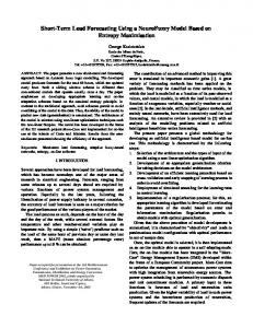
Fig 1 Load Time Series Modeling
The power system load is assumed to be time dependent evolving according to a probabilistic law. It is a common practice to employ a white noise sequences a(t) as input to a linear filter whose output is the power system load y(t). This is an adequate model for predicting the load time series. Models for time series data can have many forms. 1) The Autoregressive (AR) process: In the Autoregressive process, the current value of the time series y (t) is expressed linearly in terms of its „p‟ previous values [y (t-1), y (t-2)……. y (t-p)] and a random noise a (t). For an autoregressive process of order „p‟ i.e. AR (p), the model can be written as, y (t) = Ø1 y (t-1) +…..+ Øp y (t-p) + a (t) ---------(1) In order to write this in more convenient form the following operators are introduced. B y (t) = y (t-1); Bm y (t) = y (t-m); And A (q) = 1- Ø1 B1 – Ø2 B2 - ……- Øp Bp ; So equation (1) can be written as, A (q) y (t) = a (t) ---------(2) Where, y (t) – output or the load at time„t‟ B - Backshift operator
46
ISSN: 2319-5967 ISO 9001:2008 Certified International Journal of Engineering Science and Innovative Technology (IJESIT) Volume 1, Issue 2, November 2012 A (q) – delay polynomial Ø1… Øp – coefficients of delay polynomial p – Order of the delay polynomial a (t) – random noise. The autoregressive process in the development of AR model involves three phases: In initial model development phase techniques for preliminary identification of time series model rely on the analysis of partial autocorrelation function (pacf).For an Autoregressive process, partial autocorrelation function is useful in determination of the order of the AR model. It is as shown in Figure 1(a). The large spikes or strong correlation at k = 0 and k = 1 in the pacf figure 1(a), suggests a model with an hourly AR (2) component. Hence the Autoregressive, AR (p) model is of the form AR (2), where p = 2 is the order of the model. Sample Partial Autocorrelation Function
Sample Partial Autocorrelations
0.8
0.6
0.4
0.2
0
-0.2
0
2
4
6
8
10 Lag
12
14
16
18
20
Fig 2(A), PACF for AR (2)
In Parameter estimation phase AR (2) model calculates the coefficients of the delay polynomial A(q) using gradient based efficient estimation method i.e. Least Square method so that the energy of the noise term is minimized. Minimum forecasting error is viewed as the principal criterion in determining both model orders and its parameters. Hence the estimated value is, A (q) = 1 - 1.114B1 + 0.1165B2 -------------- (3) Once the parameters of the model have been estimated the adequacy of the model has to be tested known as the diagnostic checking. This testing procedure is performed so as to check if the parameter estimate is significantly different from zero. In this case, the model passes the above test as the parameter estimate is not equal to zero. Hence the model can be used for forecasting. In forecasting phase by using the proposed time series forecasting approach, AR (2) model is developed for hourly load data and equation (1) is used for forecasting the future load values. The Autoregressive, AR (2) model has consistently shown satisfactory performance with mean absolute percentage error (MAPE) of 13.03%. The graphs of actual load (y) in MW versus predicted load (yp) in as shown in figure 1(b) & 1(c). 9000 8000 7000 6000 5000 L oad 2012(y ) 4000
y p[A R (2)]
3000 2000 1000
1 16 31 46 61 76 91 106 121 136 151 166 181 196 211 226 241 256 271 286 301 316 331 346 361 376 391 406 421 436 451 466 481 496 511 526 541 556 571 586 601 616 631 646 661 676 691 706 721 736
0
Fig 2(B): Graph for One Month 2012 Actual Load MW (Y) Vs Predicted Load (Yp).
47
ISSN: 2319-5967 ISO 9001:2008 Certified International Journal of Engineering Science and Innovative Technology (IJESIT) Volume 1, Issue 2, November 2012 9000 8000 7000 6000 5000
L oad 2012(y )
4000
y p[A R (2)]
3000 2000 1000
162
155
148
141
134
127
120
113
99
106
92
85
78
71
64
57
50
43
36
29
22
15
8
1
0
Fig 2(C): Graph for One Week 2012 Actual Load MW (Y) Vs Predicted Load (Yp).
2) The Autoregressive Moving-Average (ARMA) Process: In the autoregressive moving average process, the current value of the time series y (t) is expressed linearly in terms of its previous „p‟ values [y (t-1), y (t-2)……..y (t-p) ] and in terms of current and previous „q‟ values of a white noise [a (t), a (t-1).…...a (t-q) ]. For an autoregressive moving average process of order „p‟ and „q‟ i.e. ARMA (p, q), the model is written as, y (t) = Ø1 y (t-1) + ……..+ Øp y (t-p) + a (t) + θ1 a (t-1) + ……. + θqa (t-q) -------------- (4) By using the backshift operator defined earlier equation (4) can be written as, A (q) y (t) = C (q) a (t) --------------- (5) Where, A(q) & C(q) – delay polynomials p & q – Orders of the delay polynomials A(q) & C(q) respectively. The autoregressive moving average process in the development of ARMA model involves three phases: In initial model development phase the partial autocorrelation function (pacf) for Autoregressive (AR) process and autocorrelation function (acf) for Moving Average (MA) process is useful in determining the orders of the ARMA model. Sample Partial Autocorrelation Function
Sample Partial Autocorrelations
0.8
0.6
0.4
0.2
0
-0.2
0
2
4
6
8
10 Lag
12
14
16
18
20
Fig 3(A), Pacf for AR (2)
The large spikes or strong correlation at k =0 and k = 1 in the pacf figure 2(a), suggests that a model with an hourly AR (2) component. Hence the Autoregressive, AR (p) model is of the form AR (2), where p = 2 is the order of the model. To facilitate the identification of the daily order or the moving average order, the multiples of 24 of the acf are inspected. Figure 2(b) suggests adding of daily moving average, MA (4) to the model because of large correlations in the acf at k = 24, 48, 72 and 96.Hence our model is of the form ARMA (2, 0) 1 * (0, 4)24, where p = 2 and q = 4 are the orders of Autoregressive and Moving Average models respectively.
48
ISSN: 2319-5967 ISO 9001:2008 Certified International Journal of Engineering Science and Innovative Technology (IJESIT) Volume 1, Issue 2, November 2012 Sample Autocorrelation Function
Sample Autocorrelation
0.8
0.6
0.4
0.2
0
-0.2
0
10
20
30
40
50 Lag
60
70
80
90
100
Fig 3(b), acf for MA (4)
In parameter tuning phase the ARMA model calculates the coefficients of A(q) and C(q) delay polynomials using Prediction error method. The estimated value of A (q) and C (q) are as given below, A (q) = 1 – 1.636B1 + 0.6357B2 ------------- (6) C (q) = 1 – 0.6313B1 – 0.04421B2 – 0.1609B3 – 0.1014B4 ------------- (7) Once the parameters of the ARMA model have been estimated, the adequacy of the model has to be tested known as the diagnostic checking. This testing procedure is performed so as to check if the parameter estimate is significantly different from zero. In this case, the ARMA model passes the above test as the parameter estimates is not equal to zero. Hence the ARMA model can be used to make forecast. In forecasting phase by using the proposed time series forecasting approach, ARMA (2, 0) 1 * (0, 4)24 model is developed for hourly load data and equation (4) is used for forecasting the future load values. The Autoregressive Moving Average, ARMA (2, 4) model has consistently shown satisfactory performance with mean absolute percentage error (MAPE) of 11.73%. The graphs of actual load (y) in MW versus predicted load (yp) in as shown in figure 2(c) & 2(d). 9000 8000 7000 6000 5000
L oad 2012(y )
4000
y p[A R MA (2,4)]
3000 2000 1000
1 15 29 43 57 71 85 99 113 127 141 155 169 183 197 211 225 239 253 267 281 295 309 323 337 351 365 379 393 407 421 435 449 463 477 491 505 519 533 547 561 575 589 603 617 631 645 659 673 687 701 715 729 743
0
Fig 3(c): Graph for one month 2012 actual load MW (y) Vs predicted load (yp).
49
ISSN: 2319-5967 ISO 9001:2008 Certified International Journal of Engineering Science and Innovative Technology (IJESIT) Volume 1, Issue 2, November 2012 9000 8000 7000 6000 5000
L oad 2012(y )
4000
y p[A R MA (2,4)]
3000 2000 1000 0 1 5 9 13172125293337414549535761656973778185899397101 105 109 113 117 1 21 125 129 133 137 141 1 45 149 153 157 161 165
Fig 3(d): Graph for one week 2012 actual load MW (y) Vs predicted load (yp).
3) The Autoregressive Integrated Moving-Average (ARIMA) Process: The time series defined previously as an AR, MA or as an ARMA process is called a stationary process. This means that the mean of the series of any of these processes and the co variances among its observations do not change with time. If the process is non-stationary, transformation of the series to a stationary process has to be performed first. This can be achieved, for the time series that are non-stationary in mean, by a differencing process. By introducing the ▼ operator, a differenced time series of order 1 can be written as, ▼y (t) = y (t) – y (t-1) = (1-B) y (t); using the definition of backshift operator, B. Consequently, an order „d‟ differenced time series is written as, ▼d y (t) = (1-B) d y (t); The differenced stationary series can be modeled as an AR, MA, or an ARMA to yield an ARIMA time series processes. For a series that needs to be differenced „d‟ times and has the orders „p‟ and „q‟ for AR and MA components i.e. ARIMA (p, d, q) model is written as, A (q) ▼d y (t) = C (q) a (t) -------------- (8) Where A (q) , ▼d , and C (q) have been defined earlier. The input series for ARIMA needs to be stationary. It should have a constant mean, variance and autocorrelation through time. Therefore, usually the series first needs to be differenced until it is stationary. In initial model development phase by looking at the autocorrelation and partial autocorrelation plots of the differenced series, we can identify the number of Autoregressive (AR) and Moving Average (MA) terms that are needed. The pacf and acf plots for differenced series are shown in figure 3(a) & 3(b). Sample Partial Autocorrelation Function
Sample Partial Autocorrelations
0.8
0.6
0.4
0.2
0
-0.2
0
2
4
6
8
10 Lag
12
14
Fig 4(a), pacf of the differenced time series
50
16
18
20
ISSN: 2319-5967 ISO 9001:2008 Certified International Journal of Engineering Science and Innovative Technology (IJESIT) Volume 1, Issue 2, November 2012 Sample Autocorrelation Function
Sample Autocorrelation
0.8
0.6
0.4
0.2
0
-0.2
0
10
20
30
40
50 Lag
60
70
80
90
100
Fig 4(b), acf of the differenced time series
The large spikes or the strong correlation at k = 0 and k = 1 in pacf in figure 3(a) suggests a model with hourly AR (2) components. Now the model AR (p) is of the form AR (2), where p = 2 is the order of the model. Hence after differencing once every 24 hours two number of Autoregressive terms are needed to build the ARIMA model. ARIMA (p, d, q) has p = 2 and d = 1.The order of Moving Average term is now to be identified by looking at the acf plot shown in figure 3(b).To facilitate the identification of the daily order or the moving average order, the multiples of 24 of the acf are inspected. Figure 3(b) suggests adding of daily moving average, MA (4) or MA (1) to the model where q = 4 or 1, because of large correlations in the acf at k=0, k= 24, k=72 & k=96. Hence four or one Moving Average term is needed to build the ARIMA model. Thus the overall ARIMA (p, d, q) takes the form ARIMA (2, 1, 4) 24 or ARIMA (2, 1, 1)24. In parameter tuning phase ARIMA (2, 1, 4)24 & ARIMA (2, 1, 1)24 model calculates the coefficients of A (q) and C (q) using prediction error method so that the energy of the noise terms is minimized. The estimated values of A (q) and C (q) are given as, A (q) = 1 + 0.09087B1 - 0.9064B2 ---------- (9) C (q) = 1 + 0.663B1 – 0.4257 B2 - 0.183 B3 – 0.08013 B4 ---------- (10) Once the parameters of the model have been estimated the adequacy of the model has been tested .The testing procedure have been performed so as to check if the parameters estimate is significantly different from zero. Here in this case the model passes the above test as the parameter estimate is not equal to zero. Hence the above ARIMA model can be used to make the forecast. In the forecasting phase by using the proposed statistical forecasting approach, ARIMA (2, 1, 4)24 & ARIMA (2, 1, 1)24 model is developed for hourly load data and equation (8) is used for forecasting the future load values. The Autoregressive Integrated Moving Average, ARIMA (2, 1, 4) 24 & ARIMA (2, 1, 1)24 model has consistently shown satisfactory performance with mean absolute percentage error (MAPE) of 6.15%. The graphs of actual load (y) in MW versus predicted load (yp) in as shown in figure 3(c) & 3(d). 9000 8000 7000 6000 5000
L oad 2012(y )
4000
yp
3000 2000 1000
1 14 27 40 53 66 79 92 105 118 131 144 157 170 183 196 209 222 235 248 261 274 287 300 313 326 339 352 365 378 391 404 417 430 443 456 469 482 495 508 521 534 547 560 573 586 599 612 625 638 651 664 677 690 703 716 729 742 755 768
0
Fig 4(c): Graph for one month 2012 actual load MW (y) Vs predicted load (yp).
51
ISSN: 2319-5967 ISO 9001:2008 Certified International Journal of Engineering Science and Innovative Technology (IJESIT) Volume 1, Issue 2, November 2012 9000 8000 7000 6000 5000
L oad 2012(y )
4000
yp
3000 2000 1000
1 4 7 10 13 16 19 22 25 28 31 34 37 40 43 46 49 52 55 58 61 64 67 70 73 76 79 82 85 88 91 94 97 100 103 106 109 112 115 118 121 124 127 130 133 136 139 142 145 148 151 154 157 160 163 166
0
Fig 4(d): Graph for one week 2012 actual load MW (y) Vs predicted load (yp).
IV. COMPARISON OF FORECASTING ERROR FOR THE DIFFERENT MODELS PROPOSED USING TIME SERIES ANALYSIS FOR SHORT TERM LOAD FORECASTING: Table 1. Summary of Obtained Results for (2011& 2012) Hourly Loads Different Models Autoregressive Model (AR) Autoregressive Moving Average Model (ARMA) Autoregressive Integrated Moving Average Model (ARIMA)
MAPE 13.03% 11.73%
6.15%
These various models tested reviews an error from 13.03% to 6.15% thus improving the performance of load forecasting model with the use of Autoregressive Integrated Moving Average with exogenous variables (ARIMAX) model. V. CONCLUSION The Short Term Load Forecasting using Time Series Analysis has been applied to Karnataka Demand pattern (2011 & 2012). The various models tested reviews an error from 13.03% to 6.15%. With Autoregressive (AR) approach the MAPE (mean absolute percentage error) is 13.03% and with Moving Average (MA) terms error reduces to 11.03%.With the Autoregressive Integrated Moving Average (ARIMA) approach the error further reduces to 6.15% indicating fairly good fit. In order to further reduce the error some exogenous variables has to be used with ARIMA model. With this Autoregressive Integrated Moving Average with exogenous variables (ARIMAX), the errors can be further reduced. Hence an attempt has been successfully made for short term load forecasting using time series analysis by developing Autoregressive (AR), Autoregressive Moving Average (ARMA) & Autoregressive Integrated Moving Average (ARIMA) models. REFERENCES [1] “Load Forecasting Bibliography”, Phase I, IEEE Transactions on Power Apparatus and Systems, Vol.PAS-99, No.1 January/February 1980. [2] “Load Forecasting Bibliography”, Phase II, IEEE Transactions on Power Apparatus and Systems, Vol.PAS-100, No.7 July 1981. [3] “The time series approach to short term load forecasting”, IEEE Transactions on Power Systems, Vol.PWRS-2, No.3 August 1987.
52
ISSN: 2319-5967 ISO 9001:2008 Certified International Journal of Engineering Science and Innovative Technology (IJESIT) Volume 1, Issue 2, November 2012 [4] “Short term load forecasting using time series modeling with peak load estimation capability”, IEEE Transactions on Power Systems, Vol.16, No.3 August 2001. [5] “Load forecasting via suboptimal seasonal autoregressive models and iteratively reweighed least squares estimation”, IEEE Transactions on Power Systems, Vol.8, No.1 February 1993. [6] “Short term load forecasting using general exponential smoothing”, IEEE Transactions on Power Systems, March/April 1971. [7]
“A real time implementation of short term load forecasting for distribution power systems”, IEEE Transactions on Power Systems, Vol.9, No.2 May 1994.
[8]
“Analysis and evaluation of five short term load forecasting techniques”, IEEE Transactions on Power Systems, Vol.4, No.4, October 1989.
[9] “Short term load forecasting, profile identification, and customer segmentation: A methodology based on periodic time series”, IEEE Transactions on Power Systems, Vol.20, No.3 August 2005. [10] “Identification of ARMAX model for short term load forecasting: An evolutionary programming approach”, IEEE Transactions on Power Systems, Vol.11, and No.1 February 1996. [11] “Neuro fuzzy approach to short term load forecasting in a price sensitive environment”, IEEE Transactions on Power Systems, Vol.17, No.4, November 2004. [12] “Short term load forecasting using fuzzy neural networks”, IEEE Transactions on Power Systems, Vol.10, No.3 August 1995. [13] “Short term load forecasting for special days in anomalous load conditions using ANN”, IEEE Transactions on Power Systems, Vol.15, No.1 February 2001. [14] “One hour ahead load forecasting using neural networks”, IEEE Transactions on Power Systems, Vol.17, No.1, February 2002. [15] “Load forecasting using support vector machines: A study on EUNITE competition 2001”, IEEE Transactions on Power Systems, Vol.19, No.4, November 2004. [16] “Composite modeling for adaptive short term load forecasting”, IEEE Transactions on Power Systems, Vol.6, No.2, May 1991. [17] “Comparison tests of fourteen distribution load forecasting methods”, IEEE Transactions on Power Systems, Vol.PAS-103, No.6, June 1984. [18] “Automated load forecasting”, IEEE Transactions on Power Systems, Vol.3, No.3, August 1988. [19] “Regressive based peak load forecasting using transformation technique”, IEEE Transactions on Power Systems, Vol.19, No.4 November 1994. [20] “Short term load forecasting for fast developing utility using knowledge-based expert systems”, IEEE Transactions on Power Systems, Vol.17, No.4, May 2002. [21] “Quantitative forecasting-The state of the explorative models”, j.opl.Res.Soc. Vol 30, No.8, 1979. [22] “Short term load forecasting”, IEEE Transactions on Power Systems, Vol.75, No.12, pp. 1558-1973, December 1987. [23] “Comparative models for electrical load forecasting”, John Wiley and Sons Ltd. 1985. [24] “Short term peak demand forecasting in fast developing utility with inherent dynamic load characteristics”, IEEE Transactions on Power Systems, Vol.5, No.3, August 1990. pp. 813-824. [25] “Short term power system load forecasting using the iteratively reweighed least squares algorithm”, Electric power system research, 19(1990) pp.11-12.
53