Shortest, Fastest, and Foremost Broadcast in Dynamic Networks ∗

January 13, 2015

9:24

WSPC/INSTRUCTION FILE

shfafo

Shortest, Fastest, and Foremost Broadcast in Dynamic Networks ∗ Arnaud Casteigts1 , Paola Flocchini2 , Bernard Mans3 , and Nicola Santoro4 1 University

of Bordeaux, France, of Ottawa, Canada, Macquarie University, Sydney, Australia, 4 Carleton University, Ottawa, Canada, 2 University

3

Highly dynamic networks rarely offer end-to-end connectivity at a given time. Connectivity in these networks can be established over time and space, based on temporal analogues of multi-hop paths (also called journeys). In a seminal work, Bui-Xuan, Ferreira, and Jarry (2003) proposed a collection of centralized algorithms to compute three types of optimal journeys in these networks – namely, shortest (min hop), fastest (min duration), and foremost (earliest arrival) journeys – given full prediction of the network evolution. We study the distributed counterparts of these problems, i.e. shortest, fastest, and foremost broadcast with termination detection (TDB), with minimal knowledge on the topology. We show that the feasibility of each variant requires distinct features on the evolution, through identifying three classes of dynamic graphs wherein the variants become gradually feasible : graphs in which the re-appearance of edges is recurrent (class R), bounded-recurrent (B), or periodic (P), together with specific knowledge that are respectively n (the number of nodes), ∆ (a bound on the recurrence time), and p (the period). To raise ambiguity, we do not require that all pairs of nodes get in contact – only a subset of them that makes the footprint of the graph connected. Our results, together with the strict inclusion between P, B, and R, implies a feasibility order among the three variants of the problem, i.e. TDB[f oremost] requires weaker assumptions on the topology dynamics than TDB[shortest], which itself requires less than TDB[f astest]. Reversely, these differences in feasibility imply that the computational powers of Rn , B∆ , and Pp also form a strict hierarchy.

Keywords: dynamic networks, distributed algorithm, time-varying graphs, delaytolerant broadcast, recurrent edges. 1. Introduction Dynamic networks are widely addressed in distributed computing. Contexts of interest are as varied as fault-tolerance, interaction scheduling, dynamic membership, planned mobility, or unpredictable mobility. The recent emergence of scenarios where entities are truly mobile and can communicate without infrastructure (e.g. vehicles, satellites, robots, or pedestrian smartphones) brought to the fore the most versatile of these environments. In these highly dynamic networks, changes are not anomalies but rather integral part of the nature of the system. The need to categorize and understand highly dynamic networks led the engineering community to design a variety of mobility models, each of which captures a particular context by means of rules that determine how the nodes move and communicate (see e.g. [23]). ∗ Preliminary

results were presented at the 6th IFIP International Conference on Theoretical Computer Science. This work has been supported in part by NSERC (Canada) and Dr. Flocchini’s University Research Chair. 1

January 13, 2015

9:24

WSPC/INSTRUCTION FILE

shfafo

2

A popular example includes the well-known random waypoint model [5]. The main interest of these models is to be able to reproduce experiments and compare different solutions on a relatively fair basis, thereby providing a common ground for the engineering community to solve practical challenges in highly dynamic networks, e.g. routing and broadcasting [8, 21, 25, 26, 28, 31, 32]. In the same way as mobility models enable to federate practical investigations in highly dynamic networks, logical properties on the graph dynamics, that is, classes of dynamic graphs, have the potential to guide a more formal exploration of their analytical aspects. A number of special classes were recently identified, for example graphs in which the nodes interact infinitely often (e.g., uniform random scheduler for population protocols [1, 2, 12]); graphs whose dynamics is unrestricted but remains connected at any instant [29, 16]; graphs in which there exists a stable connected spanning subgraph in any T-time window (a.k.a. T-interval connectivity) [27, 22]; graphs whose edges appear or disappear with given probabilities [13, 4, 14, 30]; graphs that have a stable root component [6]; graphs whose schedule is periodic [10, 18, 19, 20, 24] or guarantees minimal reachability properties [9]. These classes (among others) were organized into a hierarchy in [11]. In this paper we are interested in studying specific relationship between some of these classes, namely three subclasses of those networks called delay-tolerant networks (DTNs), in which instant connectivity is never guaranteed, but still connectivity can be achieved over time and space (see e.g. [3]). These classes are: • Class R of all graphs whose edges cannot disappear forever (recurrent edges). That is, if an edge appears once and disappears, then it will eventually re-appear at some unknown (but finite) date. It is not required that all pairs of nodes share an edge, but only that the footprint of all edges forms a connected graph (otherwise, even temporal connectivity is not guaranteed). This class corresponds to Class 6 in [11]. • Class B (for bounded-recurrent edges) consisting of those graphs with recurrent edges in which the recurrence time cannot exceed a given duration ∆. And again, the footprint is connected. This class corresponds to Class 7 in [11]. • Class P (for periodic edges) consisting of those graphs in which all topological events (appearance or disappearance) repeat identically modulo some period p. And again, the footprint is connected. This class corresponds to Class 8 in [11]. As far as inclusion is concerned, it clearly holds that P ⊂ B ⊂ R, but what about the computational relationship between these classes? Considering different types of knowledge, namely the number n of nodes in the network, a bound ∆ on the recurrence time, and (any multiple of) the period p, we look at the relationship between P(Rn ), P(B∆ ), and P(Pp ), where P(Ck ) is the set of problems one can solve in class C with knowledge k. The investigation is carried out by studying a fundamental problem in distributed computing: broadcast with termination detection at the emitter (or TDB). This problem can have at least three distinct definitions in highly dynamic networks: TDB[f oremost], in which the date of delivery is minimized at every node; TDB[shortest], where the num-

January 13, 2015

9:24

WSPC/INSTRUCTION FILE

shfafo

3

ber of hops used by the broadcast is minimized relative to every node; and TDB[f astest], where the overall duration of the broadcast is minimized (however late the departure be). These three metrics were considered in [7] as part of an offline problem where, given a complete schedule of the network, one has to compute all shortest, fastest, and foremost journeys (temporal paths) from a given node. Our contribution In this paper we examine the feasibility and reusability of the solution (and to some extent, the complexity) of TDB[f oremost], TDB[shortest], and TDB[f astest] in R and B with knowledge ∅, n, or ∆. We additionally draw some observations from external results in P with knowledge p [10], that complete our general picture of feasibility and reusability of broadcast in the three classes. Here is a short summary of the main results. Feasibility: We first show that none of these problems are solvable in any of the classes unless additional knowledge is considered. We prove constructively that knowing n makes it possible to solve TDB[f oremost] in R, but this is not sufficient to solve TDB[shortest] nor TDB[f astest], even in B. TDB[shortest] becomes in turn feasible in B if ∆ is known, but this context is not sufficient to solve TDB[f astest]; this later problem being solvable in P knowing p [10]. Put together, these results allow us to show that P(Rn ) ( P(B∆ ) ( P(Pp )

(1)

that is, the computational relationships between these three contexts form a strict hierarchy. Let us define a binary relation f easibility over problems, such that for two problems P1 and P2 , P1 f easibility P2 implies that for some class of TVG C and knowledge k we have P1 ∈ P(Ck ) while P2 ∈ / P(Ck ). This relation induces a partial order on the feasibility of problems with respect to topological changes. Our results imply that TDB[f oremost] f easibility TDB[shortest] f easibility TDB[f astest]

(2)

Reusability: Regarding the possibility to reuse a solution, that is, a same broadcast tree, over several broadcasts, we find the intriguing fact that reusability in TDB[shortest] is easier than that of TDB[f oremost]. Precisely, when TDB[shortest] becomes feasible in B, it enables at once reusability of the broadcast trees, whereas TDB[f oremost], although it was already feasible in R, does not enable reusability until in P [10]. Using a similar definition as for feasibility, we consider the relation reusability that induces a partial order over problems with respect to the reusability of a solution. Our results imply that TDB[shortest] reusability TDB[f oremost]

(3)

Whether reusability is more or less difficult in TDB[f astest] than in TDB[f oremost] is an open question, both of them being impossible in B∆ and possible in Pp . Our results on feasibility and reusability are summarized in Table 1.

January 13, 2015

9:24

WSPC/INSTRUCTION FILE

shfafo

4

Metric Foremost

Shortest

Fastest

Class R R B P R R B P R R B P

Knowledge ∅ n ∆ p ∅ n ∆ p ∅ n ∆ p

Feasibility no yes yes yes no no yes yes no no no yes

Reusability – no no yes – – yes yes – – – yes

Result from this paper this paper this paper [10] this paper this paper this paper (same result) this paper this paper this paper [10]

Table 1. Feasibility and reusability of TDB in different classes of dynamic networks (with associated knowledge).

Metric

Class Knowl.

Foremost

R B

Shortest

B

either of {

Time

Info. msgs Control msgs Info. msgs Control msgs (1st run) (1st run) (next runs) (next runs) n unbounded O(m) O(n2 ) O(m) O(n) 2 n O(n∆) O(m) O(n ) O(m) O(n) ∆ O(n∆) O(m) O(n) O(m) 0 n&∆ O(n∆)∗ O(m) 0 O(m) 0 ∆ O(n∆) O(m) O(n) : 2n − 2 O(n) 0 n&∆ O(n∆) O(m) O(n) : n − 1 O(n) 0 n&∆ O(n∆)∗ O(m) 0 O(m) 0

Table 2. Complexity of TDB for different classes of dynamic networks and associated knowledge. (The ∗ indicates that the emitter terminates implicitely, even in the first run.)

Complexity: Although complexity is not the main focus here, we characterize the time complexity and message complexity of our algorithms and observe some interesting facts. For instance, the message complexity of our algorithm to TDB[f oremost] is lower knowing ∆ than knowing n, and even lower if both are known. These results are summarized in Table 2. Note that TDB involves two processes: the actual dissemination of information messages, and the exchange of typically smaller control messages (e.g. for termination detection), both of which are separately analyzed. Regarding time complexity, we observe that for all our algorithms (except those which terminate implicitly), the termination detection phase takes the same order of time as the dissemination phase. Thus, Table 2 does not distinguish both phases.

Property 1.

January 13, 2015

9:24

WSPC/INSTRUCTION FILE

shfafo

5

2. Model and Basic Properties 2.1. Definitions and Terminology Consider a system composed of a finite set of n entities V (or nodes) that interact with each other over a (possibly infinite) time span T ⊆ T called lifetime of the system, where T is the temporal domain (typically, N or R+ for discrete and continuous-time systems, respectively). In this paper we consider a continuous-time setting with T = R+ . Following [11], we describe the network as a time-varying graph (TVG, for short) G = (V, E, T , ρ, ζ), where E ⊆ V × V is the set of m intermittently available undirected edges such that (u, v) ∈ E ⇔ u and v have at least one contact over T , ρ : E × T → {0, 1} (presence function) indicates whether a given edge is present at a given time, and ζ : E × T → T (latency function), indicates the time it takes to cross a given edge (i.e., send a message) if starting at a given time. In this paper, we assume ζ to be constant over all edges and dates, and call it the crossing delay. Thus we use the shorthand notations G = (V, E, T , ρ). Finally, the (static) graph formed by the first two elements of G, that is V and E is the footprint of G (also called underlying graph or interaction graph). This formalism essentially encompasses that of evolving graphs [17], where G is represented as a sequence of graphs G1 , G2 , ..., Gi , ... each providing a snapshot of the system at different times (which correspond either to discrete steps or topological events). In comparison, TVGs offer an interaction-centric view of the network evolution, where the evolution of each edge can be considered irrespective of the global time sequence, which turns out to be convenient when dealing with locally specified properties. A given edge e ∈ E is said to be recurrent if it appears infinitely often; that is, for any date t, ρ(e, t) = 0 =⇒ ∃t0 > t : ρ(e, t0 ) = 1. When all the edges of E are recurrent, we say that G is recurrent (keep in mind that in general E 6= V 2 ). Let R denote the class of recurrent TVGs whose footprint G = (V, E) is connected. The recurrence of an edge e is said to be time-bounded (or simply bounded), if there exists a constant ∆e such that the time between any two successive appearances of e is at most ∆e . When the recurrence of all the edges of a graph G ∈ R is time-bounded, we say that G is time-bounded recurrent, call ∆ = max{∆e : e ∈ E}, and denote by B ⊂ R the class of time-bounded recurrent TVGs. An edge e ∈ E is said to be periodic of period pe if ρ(e, t) = ρ(e, t + kpe ) for all integer k. A graph is said periodic if all its edges are periodic, and its period p is the least common multiple of all the edges periods. We denote by P ⊂ B the class of periodic TVGs. Given a TVG G = (V, E, T , ρ), we consider that G = (V, E) is always simple (no self-loop nor multiple edges) and that nodes possess unique identifiers. The set of edges being incident to a node u at time t is noted It (u) (or simply It , when the node is implicit). Finally, we note G[ta ,tb ) the temporal subgraph of a TVG G restricted to lifetime [ta , tb ). When an edge e = (x, y) appears, the entities x and y can communicate. The time ζ necessary to transmit a message (crossing delay) is known to the nodes. The minimal duration of edge presence is assumed to be 2 × ζ (i.e., long enough for a back and forth exchange of message). Algorithmically, this allows the following observations:

January 13, 2015

9:24

WSPC/INSTRUCTION FILE

shfafo

6

1. If a message is sent just after an edge has appeared, the message and a potential answer are guaranteed to be successfully transmitted. 2. If the recurrence of an edge is bounded by some ∆, then this edge cannot disappear for more than ∆ − 2 × ζ.

The appearance and disappearance of edges are instantly detected by the two adjacent nodes (they are notified of such an event without delay). If a message is sent less than ζ before the disappearance of an edge, it is lost. However, since the disappearance of an edge is detected instantaneously, and the crossing delay ζ is known, the sending node can locally determine whether the message was successfully delivered. We thus authorize the special primitive send retry as a facility to specify that if the message is lost, then it is automatically re-sent upon next appearance of the edge, and this sending is necessarily successful (Property 1). Note that nothing precludes this primitive to be called while the corresponding edge is even absent (this actually simplifies the expression of some algorithms). A sequence of couples J = {(e1 , t1 ), (e2 , t2 ), ..., (ek , tk )}, with ei ∈ E and ti ∈ T for all i, is called a journey in G iff {e1 , e2 , ...} is a walk in G and for all ti , ρ(ei )[ti ,ti +ζ) = 1 and ti+1 ≥ ti + ζ. We denote by departure(J ), and arrival(J ), the starting date t1 and last date tk + ζ of J , respectively. Journeys can be thought of as paths over time from a source node to a destination node (if the journey is finite). Let us denote by JG∗ the set of all finite journeys in a graph G. We will say that node u can reach node v in G, and note ∃J(u,v) ∈ JG∗ (or simply u v, if G is clear from the context), if there exists at least one possible journey from u to v in G. Note that the notion of journey is asymmetrical (u v tf , and the period of G 0 is some p0 > t − t0 . Consider the execution of A in G 0 starting at time t0 with x as the source. Since (u, v) does not appear from t0 to tf , the execution of A at every node in G 0 is exactly as at the corresponding node in G. In particular, node x will have entered a terminal state at time tf with node v not having received the information, contradicting the correctness of A. We thus have the following corollary, by inclusion of P. Corollary 4. TDB cannot be solved in B nor R without any additional knowledge. Hence, additional knowledge of some kind is required to solve TDB in these classes. We consider three types of knowledge, namely, the number of nodes n = |V |, an upper bound ∆ on the recurrence time (when in B), or the period p (in P). We start by establishing a general impossibility result for TDB[f astest] in B (and a fortiori in R), which cannot be solved even if both n and ∆ are known. Theorem 5. TDB[f astest] is not solvable in B (and a fortiori in R), regardless of the knowledge considered. Proof. The argument relates to the very existence of fastest journeys in an unstructured infinite setting. Consider for example the graph G = (V, E, T , ρ) ∈ B such that V = {v1 , v2 , v3 }, E = {e1 = (v1 , v2 ), e2 = (v2 , v3 )} and ρ is such that: • ∀t ∈ T , ∀i ∈ N+ , ρ(e1 , t) = 1 ⇐⇒ i∆ ≤ t < i∆ + ζ • ∀t ∈ T , ∀i ∈ N+ , ρ(e2 , t) = 1 ⇐⇒ i∆ + ζ + i−1 ≤ t < i∆ + 2ζ + i−1 for any ∆ ≥ 2ζ + 1. In such a setting, every period [i∆, (i + 1)∆) enables a journey Ji from v1 to v3 such that |Ji |t = 2ζ + i−1 . Since i−1 is decreasinga , there is an infinite sequence of journeys J1 , J2 , .. such that |Ji+1 |t < |Ji |t . a Which notation should we use among i−1 or 1/i? If the latter, please update at the four places in the proof.

January 13, 2015

9:24

WSPC/INSTRUCTION FILE

shfafo

9

Theorem 6. [10] TDB[f astest] is feasible in P with a known period p, and the solution can be reused for subsequent broadcasts. The algorithm from [10] builds fastest broadcast trees in Pp . The solution relies on learning at what time(s) in the period the temporal eccentricity of the emitter is minimum, then building a foremost broadcast tree for such date. Note that the broadcast tree so-built remains necessarily optimal in the future, since in P the whole network schedule repeats forever. It can thus be memorized for subsequent broadcasts, i.e., the solution is reusable. The rest of the paper focuses on TDB[f oremost] and TDB[shortest] in R and B, knowing n and/or ∆. We then draw some conclusions on the relative difficulty of these three problems, as well as on the computational relationship between P(Rn ), P(B∆ ), and P(Pp ). 4. TDB[f oremost] TDB[f oremost] in R or B clearly requires some sort of flooding, because the very fact of probing a neighbor to determine if it already has the information compromises the possibility to send it in a foremost fashion (in addition to risking the disappearance of the edge in-between the probe and the real sending). As a consequence of Theorem 3, this problem cannot be solved without knowledge. In this section we first show that it becomes possible in R if the number of nodes n = |V | is known. The proof is constructive by means of Algorithm 1, whose termination is however not bounded in time. Being in B with the same knowledge allows its termination to be bounded. Knowing ∆ instead of n in B then allows us to propose another solution (described in Algorithm 2) that has a lower message complexity. This complexity can be further improved if both ∆ and n are known, as in this case we have the possibility to terminate implicitly. Regarding reusability for the broadcast of the information, none of the broadcast trees built in R or even B turn out to be reusable as such, due to the inherent lack of structure of these classes. Theorem 7. Foremost broadcast trees are not reusable as such in B∆ (and a fortiori in Rn ). Proof (sketch). By contradiction, let a tree T be a reusable foremost tree with respect to emission date t. Since the order in which edges re-appear in B is arbitrary (as long as they all occur within a ∆ time window), an adversary can act on the schedule in such a way that the edges appear in a different order as that of the hierarchy of T , contradicting the fact that the tree is foremost. Note that the proof argument does not relate to the non-existence of trees whose optimality repeat in the future; in fact, there must be at least one tree whose optimality holds infinitely often since there are finitely many possible trees and infinitely many time spans of duration ∆. The argument actually relates to the non-decidability of using a given tree. Nonetheless, observe that the knowledge acquired can be helpful to lower the complexity of the termination detection.

January 13, 2015

9:24

WSPC/INSTRUCTION FILE

shfafo

10

4.1. TDB[f oremost] in R In this section we only discuss the knowledge of n since ∆ is not defined for R. 4.1.1. Knowledge of n In this section, we show how the problem is solvable when n is known. The algorithm proceeds as follows (see Algorithm 1 for details). Every time a new edge appears locally to an informed node, this node sends the information message onto this edge, and remembers that this edge now leads to an informed node. The first time a node receives the information, it records the sender as parent, transmits the information on its available edges, and sends back a notification message to the parent. Note that these notifications create a parent-relation and thus a converge-cast tree. Each notification is propagated along the converge-cast tree and eventually collected at the emitter. When the emitter has received n − 1 notifications, it knows all nodes are informed. Observe that the notification messages are sent using the special primitive send retry discussed in Section 2.1, to ensure that the parent eventually receives it even if the edge disappears during the first attempt. Information messages, on the other hand, are sent using the normal send primitive. Indeed, if the propagation of such a message fails because the corresponding edge disappears, it simply means that this edge at that particular time did not have to be used (i.e., it did not belong to a valid journey). Theorem 8. When n is known, TDB[f oremost] can be solved in R exchanging O(m) information messages and O(n2 ) control messages, in unbounded time. Proof. Since a node sends the information to each new appearing edge, it is easy to see, by connectivity of the underlying graph, that all nodes will eventually receive the information. The dissemination itself is necessarily foremost because the information is either directly relayed on edges that are present, or sent as soon as a new edge appears. As for termination detection: every node identifies a unique parent and a converge-cast spanning tree directed towards the source is implicitly constructed; since every node notifies the source (through the tree) and the source knows the total number of nodes, termination is guaranteed. Since information messages might traverse every edge in both directions, and an edge cannot be traversed twice in the same direction, we have that the number of information messages is in the worst case 2m. Since every node but the emitter induces a notification that is forwarded up the converge-cast tree to the emitter, the number of notification messages is the sum of distances in the converge-cast tree between all nodes and the emitter, P v∈V r{emitter} dh tree (v, emitter). The worst case is when the graph is a line where we 2

have n 2−n control messages. Regarding time complexity, the termination of the algorithm is unbounded due to the fact that the recurrence of the edges is itself unbounded. Reusability for subsequent broadcasts Foremost trees are time-dependent in the sense that they might be optimal for some emission dates and not be so for other dates. Still, they

January 13, 2015

9:24

WSPC/INSTRUCTION FILE

shfafo

11

Algorithm 1 Foremost broadcast in R, knowing n. 1: 2: 3: 4:

Edge parent ← nil // edge the information was received from (for non-emitter nodes). Integer nbN otif ications ← 0 // number of notifications received (for the emitter). Set inf ormedN eighbors ← ∅ // neighbors known to have the information. Status myStatus ← ¬informed // status of the node (informed or non-informed).

5:

initialization:

6: 7: 8: 9:

if isEmitter() then myStatus ← informed send(inf ormation) on Inow() onAppearance of an edge e:

10: 11: 12: 13: 14: 15: 16: 17: 18: 19: 20: 21: 22: 23: 24: 25: 26: 27:

// sends the information on all present edges.

if myStatus == informed and e ∈ / inf ormedN eighbors then send(inf ormation) on e inf ormedN eighbors ← inf ormedN eighbors ∪ {e}

// (see Prop. 1).

onReception of a message msg from an edge e: if msg.type == Inf ormation then inf ormedN eighbors ← inf ormedN eighbors ∪ {e} if myStatus == ¬informed then myStatus ← informed parent ← e send(inf ormation) on Inow() r inf ormedN eighbors // propagates. send retry(notif ication) on e // notifies that this node has the info. (this message is to be resent upon the next appearance, in case of failure). else if msg.type == N otif ication then if isEmitter() then nbN otif ications ← nbN otif ications + 1 if nbN otif ications == n − 1 then terminate // at this stage, the emitter knows that all nodes are informed. else send retry(notif ication) to parent

remain valid trees (though, possibly non-foremost ones) regardless of the considered date. As such, they can be memorized by the nodes in order to be used as converge-cast trees for termination detection in subsequent broadcasts. Indeed, while the broadcast is required to be foremost, the detection of termination does not have such constraint. Hence, instead of sending a notification each time a new node is informed (as done previously), nodes can notify their parents (in the converge-cast tree) if and only if they are themselves informed and have received a notification from each of their children (in the converge-cast tree). This reduces the number of control messages from O(n2 ) to O(n), having only one notification per edge of the converge-cast tree. 4.2. TDB[f oremost] in B If the recurrence time is bounded, then either the knowledge of n or an upper bound ∆ on the recurrence time can be used to solve the problem (with various message complexities).

January 13, 2015

9:24

WSPC/INSTRUCTION FILE

shfafo

12

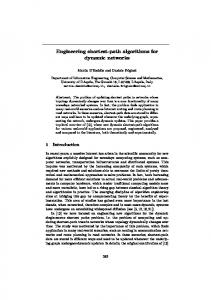
4.2.1. Knowledge of n. Since B ⊆ R, one can obviously solve TDB[f oremost] in B using Algorithm 1 (and the same observations apply regarding reusability of the converge-cast tree). Here, however, the termination time becomes bounded due to the fact that the recurrence of edges is itself bounded. Theorem 9. When n is known, TDB[f oremost] can be solved in B exchanging O(m) information messages and O(n2 ) control messages, in O(n∆) time. Proof. Since all edges in E are recurrent within any ∆ time window, the delivery of the information at the last node must occur within (n − 1)∆ global time. The same property holds for the latest notification, bounding the overall process to a duration of ∆(2n − 2). The rest follows from Theorem 8. 4.2.2. Knowledge of ∆. The information dissemination is performed as in Algorithm 1, but the termination detection is different. Thanks to the time-bound ∆ on edge recurrence, a node can discover all of its neighbors within ∆ time. This fact can be used by a node to determine whether it is a leaf in the broadcast tree (i.e., if it has not informed any other node within ∆ time following their own reception time)b . This allows the leaves to terminate spontaneously and notify their parent, which recursively terminate after receiving the notifications from all their children and notifying their own parent. With this type of termination, the whole process is in the same spirit as the Dijkstra-Scholten algorithm [15] for static graphs. In that algorithm, a particular node initiates a task that is progressively distributed over the network. The process then terminates recursively based on the relations created during the distribution, each node terminating after its children have terminated. The temporal adaption for bounded-recurrent TVGs is as follows (see Algorithm 2 for details). First, everytime a new edge appears locally to an informed node, this node sends the information on the edge, and records it. The first time a node receives the information, it chooses the sender as parent, memorizes the current time (in a variable f irstRD), transmits the information on its available edges, and returns an affiliation message to its parent using the send retry primitive (starting to build the converge-cast tree). This affiliation message is not relayed upward in the tree, but is only intended to inform the direct parent about the existence of a new child (so this parent knows it must wait for a future notification by this node). If an informed node has not received any affiliation message after a duration of ∆ + ζ, it sends a notification message to its parent using the send retry primitive. The wait is bounded by ∆ + ζ for the following reasons (see also Figure 1). First note that (due to Prop. 1) the information messages cannot be lost when they are sent on an appearing edge, neither can their potential affiliation answer. Thus, the loss of information messages can only occur when the information is directly relayed by a node which received it (say, b This

is where we need 2ζ I think...

January 13, 2015

9:24

WSPC/INSTRUCTION FILE

shfafo

13

f irstRD

+∆ +∆+ζ

a 1 b

2

3

Figure 1. Case when a node waits ∆ + ζ for receiving potential affiliation messages.

as per Figure 1, node a, relaying at time f irstRD the information to node b). As before, if the information message is lost, then it simply means that this edge at that time did not have to be used. On the other hand, if the affiliation message is lost, it must be sent again (send retry). However, in the worst case, the common edge disappears just before the affiliation message is delivered, and reappears only ∆ − 2 × ζ later (Prop. 1). Affiliation messages can thus be received until f irstRD + ∆ + ζ. If a node has one or more children, it waits until it receives a notification message from each of them, then notifies its parent in the converge-cast tree (using send retry again). Once the emitter has received a notification from each of its children, it knows that all nodes are informed. Theorem 10. When ∆ is known, TDB[f oremost] can be solved in B exchanging O(m) information messages and O(n) control message, in O(n∆) time. Proof. Correctness follows the same lines of the proof of Theorem 8. However the correct construction of a converge-cast spanning tree is guaranteed by the knowledge of ∆ (i.e., the nodes of the tree that are leaves detect their status because no new edges appear within ∆ time) and the notification starts from the leaves and is aggregated before reaching the source. The number of information messages is O(m) as the exchange of information messages is the same as in Algorithm 1, but the number of notification and affiliation messages decreases to 2(n − 1). Each node but the emitter sends a single affiliation message; as for the notification messages, instead of sending a notification as soon as it is informed, each node notifies its parent in the converge-cast tree if and only if it has received a notification from each of its children resulting in one notification message per edge of the tree. The time complexity of the dissemination itself is the same as for the foremost broadcast when n is known. The time required for the emitter to subsequently detect termination is an additional ∆ + ζ + ∆(n − 1) (the value ∆ + ζ corresponds to the time needed by the last informed node to detect that it is a leaf, and ∆(n − 1) corresponds to the worst case of the notification process, chained from that node to the emitter).

Reusability for subsequent broadcasts Clearly, the number of nodes n, which is not a priori known here, can be obtained through the notification process of the first broadcast (by having nodes reporting their number of descendants in the tree, while notifying hierarchically). All subsequent broadcasts can thus behave as if both n and ∆ were known. Next we show this allows to solve the problem without any control messages.

January 13, 2015

9:24

WSPC/INSTRUCTION FILE

shfafo

14

Algorithm 2 Foremost broadcast in B, knowing a bound ∆ on the recurrence time. 1: 2: 3: 4: 5: 6:

Edge parent ← nil // edge the information was received from (for non-emitter nodes). Integer nbChildren ← 0 // number of children. Integer nbN otif ications ← 0 // number of children that have terminated. Set inf ormedN eighbors ← ∅ // neighbors known to have the information. Date f irstRD ← nil // date of first reception. Status myStatus ← ¬informed // status of the node (informed or non-informed).

7:

initialization:

8: 9: 10: 11: 12: 13: 14: 15: 16: 17: 18: 19: 20: 21: 22: 23: 24: 25: 26: 27: 28: 29: 30: 31: 32: 33: 34: 35: 36:

if isEmitter() then myStatus ← informed send(inf ormation) on Inow() onAppearance of an edge e:

// sends the information on all present edges.

if myStatus == informed and e ∈ / inf ormedN eighbors then send(inf ormation) on e inf ormedN eighbors ← inf ormedN eighbors ∪ {e}

// (see Prop. 1).

onReception of a message msg from an edge e: if msg.type == Inf ormation then inf ormedN eighbors ← inf ormedN eighbors ∪ {e} if myStatus == ¬informed then myStatus ← informed f irstRD ← now() // memorizes the date of first reception. parent ← e send(inf ormation) on Inow() r inf ormedN eighbors // propagates. send retry(af f iliation) on e // informs the parent that it has a new child. else if msg.type == Af f iliation then nbChildren ← nbChildren + 1 inf ormedN eighbors ← inf ormedN eighbors ∪ {e} else if msg.type == N otif ication then nbN otif ications ← nbN otif ications + 1 if nbN otif ications == nbChildren then if ¬isEmitter() then // notifies the parent in turn. send retry(notif ication) to parent terminate // whether emitter or not, the node has terminated at this stage. when now() == f irstRD + ∆ + ζ:

// tests whether the underlying node is a leaf.

if nbChildren == 0 then send retry(notif ication) on parent terminate

4.2.3. Knowledge of both n and ∆ In this case, the emitter knows an upper bound on the broadcast termination date; in fact, the broadcast cannot last longer than (n − 1)∆ (this worst case is when the foremost tree is a line). Termination detection can thus become implicit after this amount of time, which removes the need for any control message (whether of affiliation or of notification).

January 13, 2015

9:24

WSPC/INSTRUCTION FILE

shfafo

15

Theorem 11. When ∆ and n are known, TDB[f oremost] can be solved in B exchanging O(m) information messages and no control messages, in O(n∆) time. 5. TDB[shortest] Let us remind that the objective of TDB[shortest] is to deliver the information to each node within a minimal number of hops from the emitter, and to have the emitter detect termination within finite time. We show below that contrary to the foremost case, knowing n is insufficient to perform a shortest broadcast in R or even in B. This becomes however feasible in B when ∆ is also known. Moreover any shortest tree built at some time t will remain optimal in B relative to any future emission date t0 > t. This feature allows the solution to TDB[shortest] to be possibly reused in subsequent broadcasts. 5.1. TDB[shortest] in B We first show that the knowledge of n is not sufficient to solve TDB[shortest] in B (and thus in R), then describe how to solve the problem when ∆ is known, and finally when both n and ∆ are known. 5.1.1. Knowledge of n The following theorem establishes that knowing n is not sufficient to solve TDB[shortest] in B (and thus in R). Theorem 12. TDB[shortest] is not feasible in B (nor a fortiori in R) knowing only n. Proof. By contradiction, let A be an algorithm that solves TDB[shortest] in B with the knowledge of n only. Consider an arbitrary G = (V, E, T , ρ) ∈ B and x ∈ V . Execute A in G starting at time t0 with x as the source. Let tf be the time when the source terminates and T the shortest broadcast tree along which broadcast was performed. Let G 0 = (V 0 , E 0 , T 0 , ρ0 ) ∈ B such that V 0 = V , E 0 = E ∪ {(x, v) for some v ∈ V : (x, v) ∈ / E}, ρ0 (e, t) = ρ(e, t) for all e ∈ E, 0 ≤ t ≤ tf , ρ0 ((x, v), t) = 0 for all t0 ≤ t < tf , and ρ0 ((x, v), t) = 1 for some t > tf (we can take ∆ as large as needed here). Consider the execution of A in G 0 starting at time t0 with x as the source. Since (x, v) does not appear between t0 and tf , the execution of A at every node in G 0 will be exactly as at the corresponding node in G and terminate with v having received the information in more than one hop, contradicting the fact that T is a shortest tree, and thus the correctness of A. 5.1.2. Knowledge of ∆ The idea is to propagate the message along the edges of a breadth-first spanning tree of the underlying graph. We present the pseudo-code in Algorithm 3, and provide the following informal description. Assuming that the message is created at some date t, the mechanism consists of authorizing nodes at level i in the tree to inform new nodes only between time t + i∆ and

January 13, 2015

9:24

WSPC/INSTRUCTION FILE

shfafo

16

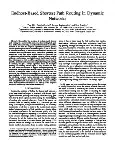
t + (i + 1)∆ (doing it sooner would lead to a non-shortest tree, while doing it later is pointless because all the edges have necessarily appeared within one ∆). So the broadcast is confined into rounds of duration ∆ as follows: whenever a node sends the information to another, it sends a time value that indicates the remaining duration of its round (that is, the starting date of its own round plus ∆ minus the current time minus the crossing delay), so the receiving node knows when to start informing new nodes in turn (if it had not the information yet). For instance in Figure 2 when the node a attempts to become b’s parent, node a transmits its own starting date plus ∆ minus the current date minus ζ. This duration corresponds to the exact amount of time the child would have to wait, if the relation is established, before integrating other nodes in turn. If a node has not informed any other node during its round, it notifies its parent. When a node has been notified by all its children, it notifies its parent. Note that this requires parents to keep track of the number of children they have, and thus children need to send affiliation messages when they select a parent (with the same constraints as already discussed in Figure 1). Finally, when the emitter has been notified by all its children, it knows the broadcast is terminated. Theorem 13. TDB[shortest] can be solved in B knowing ∆, exchanging O(m) info. messages and O(n) control messages, in O(n∆) time. Proof. The fact that the algorithm constructs a breadth-first (and thus shortest) delaytolerant spanning tree follows from the connectivity over time of the underlying graph and from the knowledge of the duration ∆. The bound on recurrence is used to enable a rounded process whereby the correct distance of each node to the emitter is detected. The number of information messages is 2m as the dissemination process exchanges at most two messages per edge. The number of affiliation and notification messages are each of n − 1 (one per edge of the tree). The time complexity for the construction of the tree is at most (n − 1)∆ to reach the last node, plus ∆ + ζ at this node, plus at most (n − 1)∆ to aggregate this node’s notification. (The additional ζ caused by waiting affiliation messages matters only for the last round, since the construction continues in parallel otherwise.) The total is thus at most (2n − 1)∆ + ζ.

roundStart

now()

roundStart + ∆

a roundStart b ζ Figure 2. Propagation of the rounds of duration ∆.

Reusability for subsequent broadcasts Thanks to the fact that shortest trees remain shortest regardless of the emission date, all subsequent broadcasts can be performed within the

January 13, 2015

9:24

WSPC/INSTRUCTION FILE

shfafo

17

same, already known tree, which reduces the number of information message from O(m) to O(n). Moreover, if the depth d of the tree is detected through the first notification process, then all subsequent broadcasts can enjoy an implicit termination detection that is itself optimal in time (after d∆ time). No control message is needed. 5.1.3. Knowledge of n and ∆ When both n and ∆ are known, one can apply the same dissemination procedure as in Algorithm 3 combined with an implicit termination detection that avoids using control messages at all. Indeed, each node learns (and possibly informs) all of its neighbors within ∆ time. Since the underlying graph is connected, the whole process must then complete within n∆ time. Hence, if the emitter knows both ∆ and n, it can simply wait n∆ time, then terminate implicitly. Theorem 14. When n and ∆ are known, TDB[shortest] can be solved in B exchanging O(m) info. messages and no control messages, in O(n∆) time. However, such a strategy would prevent the emitter from learning the depth d of the shortest tree, and thus prevent lowering the termination bound to d∆ time. An alternative solution would be to achieve explicit termination for the first broadcast in order to build a reusable broadcast tree (and learn its depth d in the process). In this case, dissemination is achieved with O(m) information messages, termination detection is achieved similarly to Algorithm 3 with O(n) control messages (where however affiliation messages are not necessary, and the number of control messages would decrease to n − 1). In this way we would have an increase in control messages, but the subsequent broadcasts could reuse the broadcast tree for dissemination with O(n) information messages, and termination detection could be implicit with no exchange of control message at all after d∆ time. The choice of either solution may depend on the size of an information message and on the expected number of broadcasts planned. 6. Computational Relationship On the basis of this paper results, we can conclude regarding the computational relationship between P(Rn ), P(B∆ ), and P(B∆ ), that is, prove the validity of Equation 1. Theorem 15. P(Rn ) ( P(B∆ ) ( P(Pp ) Proof. The fact that P(Rn ) ⊆ P(B∆ ) ⊆ P(Pp ) was observed in Theorem 2. To make the left inclusion strict, one has to exhibit a problem Π such that Π ∈ P(B∆ ) and Π∈ / P(Rn ). By Theorem 12 and Theorem 13, TDB[shortest] is one such example. The right inclusion is similarly proven strict, based on the fact that TDB[f astest] is in P(Pp ) (Theorem 6) but it is not in P(B∆ ) (Theorem 5). Now, considering the fact that TDB[f oremost] ∈ P(Rn ) while TDB[shortest] ∈ / P(Rn ), and the fact that TDB[shortest] ∈ P(B∆ ) while TDB[f astest] ∈ / P(B∆ ),

January 13, 2015

9:24

WSPC/INSTRUCTION FILE

shfafo

18

together with the inclusions of Theorem 15, we have TDB[f oremost] f easibility TDB[shortest] f easibility TDB[f astest] where f easibility is a partial order on these problems topological requirements (relative to feasibility). The order is “only” partial here because the variations of feasibility of these problems may be different in another set of assumptions. Following a similar reasoning (that is the fact that the solutions to TDB[shortest] are reusable in B∆ whereas those to TDB[f oremost] are not) leads to TDB[shortest] reusability TDB[f oremost] where reusability is a partial order on these problems topological requirements (relative to reusability). This result suggests that a problem could be both easier or more difficult than another, depending on which aspect is looked at (feasibility vs. reusability). In other words, the difficulty of these problems seems to be multi-dimensional. Finally, whether reusability is easier for TDB[f astest] or TDB[f oremost] is an open question, both of these problems being unsolvable in B∆ but solvable in Pp [10]. 7. Concluding Remarks In this paper we looked at three particular problems (shortest, fastest, and foremost broadcast) in three particular classes of dynamic graphs (recurrent, time-bounded recurrent, and periodic graphs). By comparing the feasibility of these problems within each class, we came to observe both requirement relationships between the problems and computational relationships between the classes. The methodology exploited here goes certainly beyond the scope of these problems and graph classes. In general terms, the principle here is to connect problems through their feasibility in a set of hierarchized classes of dynamic graphs. One can take two problems P1 and P2 that are respectively feasible in classes C1 and C2 , then show that both C1 ⊆ C2 and P1 is not feasible in C2 , to finally conclude that P1 is at least as difficult as P2 in terms of topological requirements. As we have shown, such characterizations can also be used reversely to exhibit computational relationship between several classes/assumptions. We hope and believe this approach could be used as a generic mean to explore further distributed algorithms in a dynamic context. Bibliography [1] D. Angluin, J. Aspnes, Z. Diamadi, M. Fischer, and R. Peralta. Computation in networks of passively mobile finite-state sensors. Distributed Computing, 18(4):235–253, 2006. [2] D. Angluin, J. Aspnes, D. Eisenstat, and E. Ruppert. The computational power of population protocols. Distributed Computing, 20(4):279–304, 2007. [3] B. Awerbuch and S. Even. Efficient and reliable broadcast is achievable in an eventually connected network. In Proceedings of the 3rd ACM symposium on Principles of distributed computing (PODC), pages 278–281, Vancouver, Canada, 1984. ACM. [4] H. Baumann, P. Crescenzi, and P. Fraigniaud. Parsimonious flooding in dynamic graphs. In Proceedings of the 28th ACM Symposium on Principles of Distributed Computing (PODC), pages 260–269, Calgary, Canada, 2009. ACM.

January 13, 2015

9:24

WSPC/INSTRUCTION FILE

shfafo

19

[5] C. Bettstetter, G. Resta, and P. Santi. The node distribution of the random waypoint mobility model for wireless ad hoc networks. IEEE Transactions on Mobile Computing, 2(3):257–269, 2003. [6] M. Biely, P. Robinson, and U. Schmid. Agreement in directed dynamic networks. In Proceedings of the 19th International Colloquium on Structural Information and Communication Complexity (SIROCCO), 2012. [7] B. Bui-Xuan, A. Ferreira, and A. Jarry. Computing shortest, fastest, and foremost journeys in dynamic networks. International Journal of Foundations of Computer Science, 14(2):267–285, April 2003. [8] J. Burgess, B. Gallagher, D. Jensen, and B.N. Levine. Maxprop: Routing for vehicle-based disruption-tolerant networks. In Proceedings of the 25th IEEE Conference on Computer Communications (INFOCOM), pages 1–11, Barcelona, Spain, 2006. IEEE. [9] A. Casteigts, S. Chaumette, and A. Ferreira. Characterizing topological assumptions of distributed algorithms in dynamic networks. In 16th Int. Colloquium on Structural Information and Communication Complexity (SIROCCO), pages 126–140, Piran, Slovenia, 2009. Springer. (Full version on arXiv:1102.5529). [10] A. Casteigts, P. Flocchini, B. Mans, and N. Santoro. Measuring temporal lags in delay-tolerant networks. IEEE Transactions on Computers, 63(2):397–410, Feb 2014. [11] A. Casteigts, P. Flocchini, W. Quattrociocchi, and N. Santoro. Time-varying graphs and dynamic networks. International Journal of Parallel, Emergent and Distributed Systems, 27(5):387–408, 2012. [12] I. Chatzigiannakis, O. Michail, and P. Spirakis. Mediated population protocols. 36th International Colloquium on Automata, Languages and Programming (ICALP), pages 363–374, 2009. [13] A. Clementi, C. Macci, A. Monti, F. Pasquale, and R. Silvestri. Flooding time in edgemarkovian dynamic graphs. In Proceedings of the 27th ACM Symposium on Principles of distributed computing (PODC), pages 213–222, Toronto, Canada, 2008. ACM. [14] A. Clementi, A. Monti, F. Pasquale, and R. Silvestri. Information spreading in stationary markovian evolving graphs. In Parallel & Distributed Processing, 2009. IPDPS 2009. IEEE International Symposium on, pages 1–12. IEEE, 2009. [15] E.W. Dijkstra and C.S. Scholten. Termination detection for diffusing computations. Information Processing Letters, 11(1):1–4, 1980. [16] C. Dutta, G. Pandurangan, R. Rajaraman, Z. Sun, and E. Viola. On the complexity of information spreading in dynamic networks. In SODA, pages 717–736, 2013. [17] A. Ferreira. Building a reference combinatorial model for MANETs. IEEE Network, 18(5):24– 29, 2004. [18] P. Flocchini, M. Kellett, P. Mason, and N. Santoro. Searching for black holes in subways. Theory of Computing Systems, 50(1):158–184, 2012. [19] P. Flocchini, B. Mans, and N. Santoro. Exploration of periodically varying graphs. In Proceedings of 20th International Symposium on Algorithms and Computation (ISAAC), pages 534–543, 2009. [20] P. Flocchini, B. Mans, and N. Santoro. On the exploration of time-varying networks. Theoretical Computer Science, 469:53–68, 2013. [21] S. Guo and S. Keshav. Fair and efficient scheduling in data ferrying networks. In Proceedings of ACM Conference on Emerging Network Experiment and Technology (CoNEXT), New York, USA, 2007. ACM. [22] B. Haeupler and F. Kuhn. Lower bounds on information dissemination in dynamic networks. arXiv preprint arXiv:1208.6051, 2012. [23] J. Harri, F. Filali, and C. Bonnet. Mobility models for vehicular ad hoc networks: a survey and taxonomy. IEEE Communications Surveys & Tutorials, 11(4):19–41, 2009. [24] D. Ilcinkas and A. Wade. On the power of waiting when exploring public transportation sys-

January 13, 2015

9:24

WSPC/INSTRUCTION FILE

shfafo

20

[25] [26]

[27]

[28] [29]

[30]

[31]

[32]

tems. Proceedings of the 15th International Conference on Principles of Distributed Systems (OPODIS), pages 451–464, 2011. P. Jacquet, B. Mans, and G. Rodolakis. Information propagation speed in mobile and delay tolerant networks. IEEE Transactions on Information Theory, 56(1):5001–5015, 2010. S. Jain, K. Fall, and R. Patra. Routing in a delay tolerant network. In Proceedings of Conference on Applications, Technologies, Architectures, and Protocols for Computer Communications (SIGCOMM), pages 145–158, 2004. F. Kuhn, N. Lynch, and R. Oshman. Distributed computation in dynamic networks. In Proceedings of the 42nd ACM Symposium on Theory of Computing (STOC), pages 513–522, Cambridge, USA, 2010. ACM. C. Liu and J. Wu. Scalable routing in cyclic mobile networks. IEEE Transactions on Parallel and Distributed Systems, 20(9):1325–1338, 2009. R. O’Dell and R. Wattenhofer. Information dissemination in highly dynamic graphs. In Proceedings of the Joint Workshop on Foundations of Mobile Computing (DIALM-POMC), pages 104–110, Cologne, Germany, 2005. ACM. Y. Peres, A. Sinclair, P. Sousi, and A. Stauffer. Mobile geometric graphs: Detection, coverage and percolation. In Proceedings of the Twenty-Second Annual ACM-SIAM Symposium on Discrete Algorithms, pages 412–428. SIAM, 2011. Z. Zhang. Routing in intermittently connected mobile ad hoc networks and delay tolerant networks: Overview and challenges. IEEE Communications Surveys & Tutorials, 8(1):24–37, 2006. W. Zhao, M. Ammar, and E. Zegura. A message ferrying approach for data delivery in sparse mobile ad hoc networks. In Proceedings of the 5th ACM International Symposium on Mobile Ad Hoc Networking and Computing (MOBIHOC), pages 187–198, 2004.

January 13, 2015

9:24

WSPC/INSTRUCTION FILE

shfafo

21

Algorithm 3 Shortest broadcast in B, knowing a bound ∆ on the recurrence.

6:

Edge parent ← nil // edge the information was received from (for non-emitter nodes). Date roundStart ← +∞ // date when the underlying node starts informing new nodes. Set children ← ∅ // set of children from which a notification is expected. Integer nbN otif ications ← 0 // number of children that have sent their notification. Set inf ormedN eighbors ← ∅ // set of neighbors known to have the info. Status myStatus ← ¬informed // status of the node (informed or non-informed).

7:

initialization:

1: 2: 3: 4: 5:

8: 9:

10: 11: 12: 13: 14: 15: 16: 17: 18: 19: 20: 21: 22: 23: 24: 25: 26: 27: 28: 29: 30:

if isEmitter() then roundStart ← now() now() == roundStart:” (below) to execute.

// causes the procedure ”when

onAppearance of an edge e: if myStatus == informed then if e ∈ / inf ormedN eighbors then send(roundStart + ∆ − now() − ζ) on e // time until the end of the round. inf ormedN eighbors ← inf ormedN eighbors ∪ {e} // (see Prop. 1). onReception of a message msg from an edge e: if msg.type == Duration then inf ormedN eighbors ← inf ormedN eighbors ∪ {e} if parent == nil then parent ← e roundStart ← now() + msg send retry(af f iliation) on e else if msg.type == Af f iliation then children ← children ∪ {e} else if msg.type == N otif ication then nbN otif ications ← nbN otif ications + 1 if nbN otif ications == |children| then if ¬isEmitter() then send retry(notif ication) on parent terminate when now() == roundStart:

myStatus ← informed 32: send(∆-ζ) on Inow() r inf ormedN eighbors // nodes that receive this message and have no parent yet will take this node as parent and wait ∆-ζ before informing new nodes. 31:

33: 34: 35:

when now() == roundStart + ∆ + ζ: // tests whether the underlying node is a leaf. if |children| == 0 then send retry(notif ication) on parent